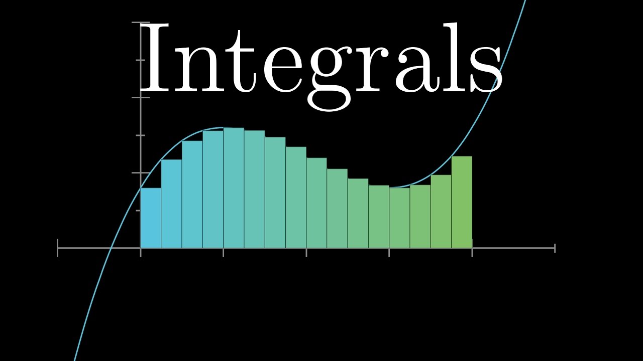
What does area have to do with slope?

We often hear that mathematics consists mainly of "proving theorems." Is a writer's job mainly that of "writing sentences?"

— Gian-Carlo Rota

Here, I want to discuss one common type of problem where integration comes up: Finding the average of a continuous variable.

This is a useful thing to know in its own right, but what's really neat is that it gives a completely different perspective for why integrals and derivatives are inverses of each other.

Quick Intuition

Before jumping into the main line of reasoning, the way this works is to take the area under the curve, and divide it by the width of that region. You might imagine that area as a pile of sand, and if you shake it all down to be flat, i.e. forming a rectangle whose area matches the area under the curve, the height of that rectangle should be the the average height of the function. To calculate that height, you would take the area of the rectangle and divide by its width.

This is intuitive, but you might find it worthwhile to also think about how this relates to the more familiar method of averaging finitely many numbers, which is to add them all up and divide by how many there are. A very common feeling is that when you use a sum in a discrete context, you use an integral in a continuous context. But to avoid subtle errors in making this translation, its useful to be able to think exactly how and why the analogy from sums to integrals works in various contexts where it comes up. This question of finding the average value of a function offers a great chance to exercise that muscle.

Average of sine function

Take a look at the graph of \sin(x) between 0 and \pi, which is half its period.

What is the average height of this graph on that interval? It's not a useless question. All sorts of cyclic phenomena in the world are modeled with sine waves: For example, the number of hours the sun is up per day as a function of which-day-of-the-year-it-is follows a sine wave pattern.

If you wanted to predict, say, the average effectiveness of solar panels in summer months vs. winter months, you'd want to be able to answer a question like this: What's the average value of that sine function over half its period.

Whereas a case like that will have all sorts of constants mucking up the function, we'll just focus on an unencumbered \sin(x) function, but the substance of the approach would be the same in any application.

It's kind of a weird thing to think about, isn't it, the average of a continuous variable. Usually, with averages, we think of a finite number of values, where you add all of them up and divide that sum by how many values there are. But there are infinitely many values of \sin(x) between 0 and \pi, and it's not like we can add all those numbers and divide by infinity.

This sensation actually comes up a lot in math, and is worth remembering, where you have this vague sense that you want to add together infinitely many values associated with a continuum, even though that doesn't really make sense. Almost always, when you get this sense, the key will be to use an integral somehow. And to think through exactly how, a good first step is usually to approximate your situation with some kind of finite sum.

In this case, imagine sampling a finite number of points, evenly spaced in this range.

Since it's a finite sample, you can find the average by adding up all the heights, \sin(x), at each one, and divide that sum by the number of points you sampled, right?

And presumably, if the idea of an average height among all infinitely many points is going to make any sense at all, the more points we sample, which would involve adding up more heights, the closer the average of that sample should be to the actual average of the continuous variable.

This should feel at least somewhat related to taking an integral of \sin(x) between 0 and \pi, even if it might not be clear at first exactly how the two ideas will match up.

\int_0^\pi \sin (x) d x

For that integral, you also think of a sample of inputs on this continuum, but instead of adding the height \sin(x) at each one, and dividing by how many there are, you add up \sin(x) \cdot dx where dx is the spacing between the samples; that is, you're adding little areas, not heights.

Technically, the integral is not quite this sum, it's whatever that sum approaches as dx approaches 0. But it's helpful to reason with respect to one of these finite iterations, where you're adding the areas of some specific number of rectangles. So what you want to do is reframe this expression for the average, this sum of the heights divided by the number of sampled points, in terms of dx, the spacing between samples.

\text { (Number of samples) } \approx \frac{x_2 - x_1 }{dx}

For example, if the spacing between these points is 0.1, and you know that they range from 0 to \pi, then you can take the length of the interval, \pi, and divide it by the length of the space between each sample. If it doesn't go in evenly, you'd round down to the nearest integer, but as an approximation this is fine.

\text { (Number of samples }) \approx \frac{\pi}{0.1} \approx 31

If we write the spacing between samples as dx, the number of samples is \frac{\pi}{dx}. So replacing the denominator with \frac{\pi}{dx} here, you can rearrange, putting the dx up top and distributing.

But, think about what it means to distribute that dx up top; it means the terms you're adding all look like \sin(x) \cdot dx for the various inputs x that you're sampling, so that numerator looks exactly like an integral expression. And for larger and larger samples of points, this average approaches the actual integral of \sin(x) between 0 and \pi, all divided by the length of that interval, \pi.

In other words, the average height of this graph is this area divided by its width. On an intuitive level, and just thinking in terms of units, that feels pretty reasonable, doesn't it? Area divided by width gives you average height.

Computing a result

Let's actually compute this integral expression. As we saw, last lesson, to compute an integral you need to find an antiderivative of the function inside the integral; some function whose derivative is \sin(x). And, if you're comfortable with trig derivatives, you know the derivative of \cos(x) is -\sin(x).

If you negate that, -\cos(x) is the antiderivative of \sin(x).

To gut check yourself on that, look at this graph of -\cos(x). At 0, the slope is 0, then it increases to some maximum slope at \pi/2, then it goes back down to 0 at \pi, and in general its slope does indeed seem to match the height of the sine graph.

To evaluate the integral of \sin(x) between 0 and \pi, take that antiderivative at the upper bound, and subtract its value at the lower bound.

\int_0^\pi \sin (x) d x=(-\cos (\pi))-(-\cos (0))

More visually, that's the difference in the height of this -\cos(x) graph above \pi, and its height at 0, and as you can see, that change in height is exactly 2.

That's kind of interesting, isn't it? That the area under this sine graph turns out to be exactly 2.

The answer to our average height problem, this integral divided by the width of the region, evidently turns out to be \frac{2}{\pi}, which is around 0.64.

\frac{\int_0^\pi \sin (x) d x}{\pi-0}=\frac{(-\cos (\pi))-(-\cos (0))}{\pi-0}=\frac{2}{\pi} \approx 0.64

Comprehensive Question

Now is a good time to try your hand at calculating the average value of a function over a range. For example, given the function f(x)=-x^2+4 x-3, what is the average value of the function between 1 and 3?

Another perspective

I promised at the start that this question of finding the average value of a function offers an alternate perspective on on why integrals and derivatives are inverses of one and other; why the area under one graph is related to the slope of another.

Notice how finding this average value \frac{2}{\pi} came down to looking at the change in the antiderivative -\cos(x) over the input range, divided by the length of that input range. Another way to think about that fraction is as the rise-over-run slope between the point of the antiderivative graph below zero, and the point of that graph above \pi.

Now think about why it might make sense that this slope represents the average value of \sin(x) on that region. By definition, \sin(x) is the derivative of this antiderivative graph; it gives the slope of -\cos(x) at every input. So another way to think about the average value \sin(x) is as the average slope over all tangent lines here between 0 and \pi. And from that view, doesn't it make a lot of sense that the average slope of a graph over all its point in a certain range should equal the total slope between the start and end point?

Generalize this view

To digest this idea, it helps to see what it looks like for a general function. For any function f(x), if you want to find its average value on some interval, say between a and b, what you do is take the integral of f on that interval, divided by the width of the interval.

You can think of this as taking the area under the graph divided by the width. Or more accurately, it's the signed area of that graph, since area below the x-axis is counted as negative.

And take a moment to remember the connection between this idea of a continuous average and the usual finite notion of an average, where you add up many numbers and divide by how many there are. When you take some sample of points spaced out by dx, the number of samples is about the length of the interval divided by dx.

If you add up the value of f(x) at each sample and divide by the total number of samples, it's the same as adding up the products f(x) \cdot dx and dividing by the width of the entire interval.

The only difference between that and the integral expression is that the integral asks what happens as dx approaches 0, but that just corresponds with samples of more and more points that approximate the true average increasingly well. Like any integral, evaluating this comes down to finding an antiderivative of f(x), commonly denoted capital F(x).

In particular, what we want is the change to this antiderivative between a and b, F(b) - F(a), which you can think of as the change in the height of this new graph between the two bounds.

I've conveniently chosen an antiderivative which passes through 0 at the lower bound here, but keep in mind that you could freely shift this up and down, adding whatever constant you want to it, and it would still be a valid antiderivative. So the solution to the average problem is the change in the height of this new graph divided by the change to its x value between a and b.

\frac{\displaystyle \int_a^b f(x) d x}{b-a}=\frac{F(b)-F(a)}{b-a}

In other words, it's the slope of the antiderivative graph between these endpoints.

And again, that should make a lot of sense, because little f(x) gives the slope of a tangent line to this graph at each point, after all it is by definition the derivative of capital F.

Why are antiderivative the key to solving integrals? Well, my favorite intuition is still the one I showed last lesson, but a second perspective is that when you reframe the question of finding the average of a continuous value as finding the average slope of bunch of tangent lines, it lets you see the answer just by the comparing endpoints, rather than having to actually tally up all points in between.

Summary

In the last video, I described a sensation that should bring integrals to your mind. Namely, if you feel like the problem you're solving could be approximated by breaking it up somehow, and adding up a large number of small things. Here I want you to come away recognizing a second sensation that should bring integrals to your mind. If there's some idea that you understand in a finite context, and which involves adding up multiple values, like taking the average of a bunch of numbers, and if you want to generalize that idea to apply to an infinite continuous range of values, try seeing if you can phrase things in terms of an integral. It's a feeling that comes up enough that's it's definitely worth remembering.