How colliding blocks act like a beam of light...to compute pi.
The third and final part of the block collision sequence.
You know that feeling when you have two mirrors facing each other, and it gives the illusion of there being an infinite tunnel of rooms? If they're at an angle with each other, it makes you feel like you're part of a strange kaleidoscopic world with many copies of yourself all separated by angled pieces of glass. What many people may not realize is that the idea underlying this illusion can be quite helpful for solving serious problems in math.

We've already had two lessons describing the block collision problem with its wonderfully surprising answer. Big block comes in from the right, lots of clacks, the total number of clacks looks like \pi, and we want to know why.
Here we see one more perspective explaining what's going on, where—as if the connection to \pi wasn't surprising enough—we add one more unexpected connection to optics.
But we're doing more than just answering the same question twice. This alternate solution gives a richer understanding that can let you answer other questions about the setup, and it's also core to how I coded accurate simulations of these blocks without requiring absurdly small time steps and huge computation time.
Position Phase Space
Last time we used a coordinate plane where each point encodes a pair of velocities. Here, we use a coordinate plane where each point encodes the positions of both blocks. Again, the idea is that by representing the states of a changing system with individual points in some space, problems in dynamics turn into problems in geometry, which are hopefully more solvable.
Specifically, let the x-coordinate of a 2D plane represent the distance from the wall to the left edge of the first block, which I'll call \textcolor{green}{d_1}. And let the y-coordinate represent the distance from the wall to the right edge of the second block, which I'll call \textcolor{red}{d_2}.

That way, the line x = y shows us where the two blocks clack into each other, since that happens whenever \textcolor{green}{d_1} = \textcolor{red}{d_2}.

Here's what it looks like for our scenario to play out:
As the two distances of our blocks change, the two-dimensional point of our configuration space moves around, with a position that always fully encodes the information of those two distances.
You may notice that at the bottom there, it's bounded by the line where \textcolor{red}{d_2} is the same as the small block's width, which is what it means for the small block to hit the wall.
You might be able to guess where we're going with this: The way this point bounces between these two bounding lines is a bit like light bouncing between two mirrors. The analogy doesn't quite work, though. In the lingo of optics, the angle of incidence doesn't equal the angle of reflection.

Just think of that first collision: If the line x = y behaved like a mirror, then a beam of light coming in from the right would bounce off this 45-degree x = y line and end up going straight down, which would mean the first block stops moving entirely.

This does actually happen in the simplest case, where the second block has the same mass as the first and picks up all of the momentum like a croquet ball. But for any other mass ratio, that first block will keep moving a bit, so the trajectory of our point in this configuration space won't be pointed straight down.
Even if it's not immediately clear why this analogy with light would be helpful, run with me for a moment and see if we can fix it for the general case, because analogies like these are often very useful when working on a difficult math problem.
Fixing the Light Analogy
Just like in the previous lesson, it's helpful to rescale the coordinates. In fact, motivated by what we did then, you might think to rescale the coordinates so that x = \sqrt{\textcolor{blue}{m_1}} \textcolor{green}{d_1}. This has the effect of stretching our space horizontally, so changes to our big block's position now result in larger changes to the x-coordinate of our point. Likewise, let's write the y-coordinate as y = \sqrt{\textcolor{blue}{m_2}} \textcolor{green}{d_2}, even though in this particular case that second mass is 1, so it doesn't matter.

Rescaling our x and y coordinates stretches everything out horizontally.
Maybe that strikes you as making things uglier, and like a somewhat random thing to do, but as with last time, when we include square roots of masses like this, everything plays more nicely with the laws of conserving energy and momentum.
Specifically, the conservation of energy will translate to the fact that our little point in configuration space is always moving at the same speed, which in our analogy you might think of as meaning there's a constant speed of light. And the conservation of momentum will translate to the fact that as our point bounces off the "mirrors" of our setup, the angle of incidence equals the angle of reflection.
Doesn't that seem bizarre? That the laws of mechanics should translate to laws of optics like this?

To see why this is true, let's roll up our sleeves and work out the math.
Understanding the Conservation Laws
Focus on the velocity vector for our point in the diagram, showing which direction it's moving and how quickly.

Note, this is not a physical velocity, like the velocities of the moving blocks; instead it's a more abstract rate of change in the context of our configuration space, whose two dimensions worth of possible directions encode the velocities of both of the blocks.
The x-component of this little vector is the rate of change of x. Likewise, its y-component is the rate of change for y.

But what is the rate of change for the x-coordinate? Well, x = \sqrt{\textcolor{blue}{m_1}}\textcolor{green}{d_1}, and the mass doesn't change, so it depends only on how \textcolor{green}{d_1} changes. And the rate at which \textcolor{green}{d_1} changes is just the velocity of the big block, which I'll call \textcolor{green}{v_1}. So \frac{dx}{dt} = \sqrt{\textcolor{blue}{m_1}}\textcolor{green}{v_1}. Likewise, the rate of change for y is \frac{dy}{dt} = \sqrt{\textcolor{blue}{m_2}}\textcolor{red}{v_2}.
Now we can calculate the magnitude of this little configuration-space-change-vector. Using the pythagorean theorem…

So the speed of our point in configuration space is based on the kinetic energy of the system. And since that energy is constant, the speed also stays constant throughout the process. Remember, a core assumption here is that no energy is lost to friction or to the collisions.
Alright, that's cool. With these rescaled coordinates our little point always moves with a constant speed. I know it's not obvious why you'd care, but among other things, it's important for the next step, where the conservation of momentum implies that these two bounding lines act like mirrors.
But first, let's understand this line \textcolor{green}{d_1} = \textcolor{red}{d_2} a little bit better. In our new coordinates, it's no longer a nice 45-degree x = y line.

Instead, after a little rearrangement, we can see that it looks like the line \frac{x}{\sqrt{\textcolor{blue}{m_1}}} = \frac{y}{\sqrt{\textcolor{blue}{m_2}}}, which is a line with slope \frac{\sqrt{\textcolor{blue}{m_2}}}{\sqrt{\textcolor{blue}{m_1}}}. That's a nice expression to tuck away in the back of your mind.
\frac{\sqrt{\textcolor{blue}{m_2}}}{\sqrt{\textcolor{blue}{m_1}}}
After the blocks collide, meaning our point hits this line, the way to figure out how they move is to use the conservation of momentum, which says the value \textcolor{blue}{m_1}\textcolor{red}{v_1} + \textcolor{blue}{m_2}\textcolor{red}{v_2} remains unchanged after the collision.

Notice, this looks like a dot product between two column vectors:
\begin{align*}
\textcolor{blue}{m_1}\textcolor{red}{v_1} + \textcolor{blue}{m_2}\textcolor{red}{v_2} &= \text{const.} \\[1em]


\begin{bmatrix}
\textcolor{blue}{m_1} \\
\textcolor{blue}{m_2}
\end{bmatrix}

\cdot

\begin{bmatrix}
\textcolor{red}{v_1} \\
\textcolor{red}{v_2}
\end{bmatrix}
&= \text{const.}
\end{align*}
And since we're interested in how this relationship will play out with our rescaled coordinates, we can rework the dot product to use the rates of change of x and y:
\begin{align*}
\textcolor{blue}{\sqrt{m_1}}\underbrace{(\textcolor{blue}{\sqrt{m_1}}\textcolor{red}{v_1})}_{dx/dt} +
\textcolor{blue}{\sqrt{m_2}}\underbrace{(\textcolor{blue}{\sqrt{m_2}}\textcolor{red}{v_2})}_{dy/dt}
&= \text{const.}

\\[2em]


\begin{bmatrix}
\textcolor{blue}{\sqrt{m_1}} \\
\textcolor{blue}{\sqrt{m_2}}
\end{bmatrix}

\cdot

\begin{bmatrix} dx/dt \\ dy/dt \end{bmatrix}
&= \text{const.}
\end{align*}
I know this probably seems like a complicated way to talk about a simple momentum equation, but there is a good reason for shifting to a language of dot products in our new coordinates.
Notice that the vector containing the derivatives is really just the velocity vector for the point in our diagram that we've been looking at.

And the other vector, with the square roots of the masses, has a representation in this diagram too. It points in the same direction as our collision line, since we found earlier that the slope of that line is \frac{\sqrt{\textcolor{blue}{m_2}}}{\sqrt{\textcolor{blue}{m_1}}}.

If you're unfamiliar with the dot product, I do have , but real quick let's review what it means geometrically. The dot product of two vectors equals the length of the first, time the length of the projection of the second one onto that first (considered negative if they point in opposite directions). You often see this written as the product of the lengths of each vector times the cosine of the angle between them.

Alright, so look back at this conservation of momentum expression, which tells us that this dot product stays constant before and after the collision:
\begin{bmatrix}
\textcolor{blue}{\sqrt{m_1}} \\
\textcolor{blue}{\sqrt{m_2}}
\end{bmatrix}

\cdot

\begin{bmatrix} dx/dt \\ dy/dt \end{bmatrix}
= \text{const.}
Since we just saw that this rate-of-change vector has a constant magnitude, and the masses never change, the only way for this dot product to stay the same is if the angle it makes with that collision line stays the same.

Similarly, when the small block bounces off the wall, our little vector gets reflected about the x-direction, since only its y-coordinate changes. So our configuration point is bouncing off that horizontal line as if it was a mirror.

Step back for a moment and think about what this means for our original question of counting block collisions. We can now translate the collision count question into a different question entirely, this time in the world of optics.
Given our coordinate setup, what question could we ask that would give us the number of block collisions, but which only involves optics, not blocks?
Unfolding the Mirror
Now I can hear some of you complaining: "Haven't we replaced one tricky setup with another?". This might make for a cute analogy, but how is it progress? It's true; counting the number of light bounces here is hard. But now we have a helpful trick.
When the beam of light hits the mirror, instead of thinking of the beam as reflecting about the mirror, think of the beam as going straight while the whole world gets flipped. It's as if the beam is passing through a piece of glass into an illusory "looking glass universe."

Instead of the light bouncing off the mirror, imagine it passing straight through into a flipped world.
Think of actual mirrors here. The wire on the left will represent a laser beam coming into the mirror, while the one on the right will represent its reflection:

The illusion is that the beam goes straight through the mirror, as if passing through a window separating us from another room.
But notice! Crucially! For this illusion to work, the angle of incidence has to equal the angle of reflection. Otherwise the flipped copy of the reflected beam won't line up with the first part.

If the angles of incidence and reflection don't match, then the illusion of passing straight through to a flipped world doesn't work.
So all that work we did rescaling coordinates and futzing through the momentum equation was certainly necessary. Now we get to enjoy the fruits of our labor. This helps us elegantly solve the question of how many mirror bounces there will be, which is also the question of how many block collisions there will be.
Every time the beam hits a mirror, don't think of the beam as getting reflected. Let it continue straight while the world gets reflected.
As this goes on, the illusion to the light beam is that instead of getting bounced around between these two angled mirrors many times, it's passing through a sequence of angled pieces of glass, all the same angle apart.
Let's compare the original bouncing beam to the illusory straight one.
Our original question of counting bounces turns into a question about how many pieces of glass this illusory beam crosses. How many reflected copies of the world does it pass into?
Well, calling the angle between the mirrors theta, the answer here is however many times you can add theta to itself without going more than halfway around the circle (so the sum must be less than \pi total radians).
Written as a formula, the answer to our question is the floor of \pi divided by \theta, \left\lfloor \frac{\pi}{\theta} \right\rfloor.
Summary
Let's review! We started by drawing a configuration space for our colliding blocks, where the x and y coordinates represented the two distances from the wall.
This kind of looked like light bouncing between two mirrors, but to make the analogy work properly, we needed to rescale the coordinates by the square roots of the masses. This made the slope of one line \frac{\sqrt{\textcolor{blue}{m_2}}}{\sqrt{\textcolor{blue}{m_1}}}.
So the angle between our two bounding lines will be the inverse tangent of the slope, \theta = \arctan(\sqrt{\frac{m_2}{m_1}}).

To figure out how many bounces there are between two mirrors like this, think of the illusion of the beam continuing straight through a sequence of looking glass universes separated by a semicircular fan of windows.

The answer, then, comes down to how many times the value of \theta fits into \pi radians.
From here, to understand why exactly the digits of \pi show up, when the mass ratio is a power of 100, it's exactly what we did in the , so I won't repeat myself here.
Final thoughts
As we reflect on how absurd the initial appearance of \pi seemed, on the two solutions we've now seen, and on how unexpectedly helpful it can be to represent the state of your system with points in some space, I leave you with this quote from computer scientist Alan Kay:
A change of perspective is worth 80 IQ points.— Alan Kay
Thanks
Special thanks to those below for supporting this lesson.