Cross products in the light of linear transformations
The formula for the cross product can feel like a mystery, or some kind of crazy coincidence. But it isn't. There is a fundamental connection between the cross product and determinants.
From [Grothendieck], I have also learned not to take glory in the difficulty of a proof: difficulty means we have not understood. The idea is to be able to paint a landscape in which the proof is obvious.
- Pierre Deligne
In the last chapter, we talked about how to compute a three-dimensional cross product of two vectors, \vec{\mathbf{v}} \times \vec{\mathbf{w}}. It's this funny thing where you write a matrix whose second column has the coordinates of \vec{\mathbf{v}}, whose third columns has the coordinates of \vec{\mathbf{w}}, but the entries of the first column, weirdly, are the basis vectors \hat{\imath}, \hat{\jmath} and \hat{k}, where you pretend they are numbers for the sake of computations.
\left[\begin{array}{l}v_1 \\v_2 \\v_3\end{array}\right] \times\left[\begin{array}{l}w_1 \\w_2 \\w_3\end{array}\right]=\operatorname{det}\left(\left[\begin{array}{lll}\hat{\imath} & v_1 & w_1 \\\hat{\jmath} & v_2 & w_2 \\\hat{k} & v_3 & w_3\end{array}\right]\right)If you just chug along with the computation, ignoring this weirdness, you get some constant times \hat{\imath}, plus some constant times \hat{\jmath}, plus some constant times \hat{k}, which defines a new 3d vector.
\vec{\mathbf{p}} = \hat{\imath} \underbrace{\left(v_2 w_3-v_3 w_2\right)}_{\text {Some number }}+\hat{\jmath} \underbrace{\left(v_3 w_1-v_1 w_3\right)}_{\text {Some number }}+\hat{k} \underbrace{\left(v_1 w_2-v_2 w_1\right)}_{\text {Some number }}
From here, students are typically told to just believe that the resulting vector has the following geometric properties:
- Its length equals the area of the parallelogram defined by
\vec{\mathbf{v}}and\vec{\mathbf{w}}. - It points in a direction perpendicular to
\vec{\mathbf{v}}and\vec{\mathbf{w}}, - This direction obeys the right-hand rule, in the sense that if you point your forefinger along
\vec{\mathbf{v}}, and your middle finger along\vec{\mathbf{w}}, then stick out your thumb, it will point in the direction of the new vectors.

There are some brute-force computational ways to confirm these facts, but I want to share with you a really elegant line of reasoning. This leverages a bit of background, though, so I'm assuming everyone has read on the determinant, and where I introduce the idea of duality. So, you know, go back and take a look if needed.
Under the light of transformations
As a reminder, the idea of duality is that anytime you have a linear transformation from some space to the number line, it is associated with a unique vector in that space, in the sense that performing the linear transformation is the same as taking a dot product with that vector.

Any time you have a 2d-to-1d linear transformation it's associated with some vector.
Numerically, it's because one of those transformations is described by a matrix with just one row, where each column tells you which number the basis vectors land on. And multiplying this matrix by some vector \vec{\mathbf{v}} is computationally identical to taking the dot product between \vec{\mathbf{v}} and the vector you get by turning that matrix on its side.

The takeaway is that when you're out in the mathematical wild and you find a linear transformation to the number line, you will be able to match it to some vector, which is called the "dual vector" of the transformation, so that performing that linear transformation is the same as taking the dot product with that vector.
The idea
The cross product gives us a really slick example of this process in action. It takes some effort, but it's definitely worth it. What I'm going to do is define a certain linear transformation from three dimensions to the number line, and it will be defined in terms of two vectors \vec{\mathbf{v}} and \vec{\mathbf{w}}. Then, when we associate that transformation with its dual vector in 3d space, that dual vector will be the cross product of \vec{\mathbf{v}} and \vec{\mathbf{w}}. Understanding that transformation will make clear the connection between the geometry and the computation of the cross product.

To back up a bit, remember that in two dimensions, computing the 2d version of the cross product of vectors \vec{\mathbf{v}} and \vec{\mathbf{w}} involves taking the determinant of a matrix whose columns contain the coordinates of those vectors. There's no nonsense with basis vectors stuck in the matrix, just an ordinary determinant returning a number. Geometrically, this gives us the area of the parallelogram spanned out by those two vectors, with the possibility of being negative depending on the orientation of the vectors.

If you didn't already know the 3d cross product, you might imagine that it involves taking 3 separate 3d vectors, \vec{\mathbf{u}}, \vec{\mathbf{v}}, and \vec{\mathbf{w}}, making their coordinates the columns of a 3x3 matrix, and computing the determinant of that matrix. As you know from , geometrically this would give the volume of a parallelepiped spanned out by those 3 vectors, with the plus or minus sign of your result depending on their right-hand rule orientation of the three vectors.

Of course, you all know this is not the 3d cross product, since the actual 3d cross product takes two vectors and spits out a vector, it doesn't take in three vectors and spit out a number. But this idea actually gets us really close to what the real cross product is. Consider the first vector \vec{\mathbf{u}} to be a variable, while \vec{\mathbf{v}} and \vec{\mathbf{w}} are fixed.

What we have, then, is a function from three dimensions to the number line. You input some vector \vec{\mathbf{u}}, and you get a number by taking the determinant of a matrix whose first column is \vec{\mathbf{u}}, and whose other two columns are the constant vectors \vec{\mathbf{v}} and \vec{\mathbf{w}}. Geometrically, the meaning of this function is that for any input vector \vec{\mathbf{u}}, you consider the parallelepiped defined by this vector, \vec{\mathbf{v}} and \vec{\mathbf{w}}, then return its volume, with a plus or minus sign depending on orientation. What's more, this function is linear.

So here we are, out in the mathematical wild with a linear transformation that outputs numbers. The idea of duality should be perking up in your mind. What we're going to do is find the matrix that describes this transformation, which will be a 1x3 matrix since the transformation goes from three dimensions to one. In other words, we're looking for a 1x3 matrix such that multiplying this matrix by some vector \vec{\mathbf{u}} gives the same result as plugging in \vec{\mathbf{u}} to the first column of a 3x3 matrix whose other two columns have the coordinates of \vec{\mathbf{v}} and \vec{\mathbf{w}}, and computing the determinant.

If you think in terms of duality and turn this matrix on its side, we're looking for a special 3d vector, that I'll call \vec{\mathbf{p}}, such that taking the dot product between \vec{\mathbf{p}} and any other vector \vec{\mathbf{u}} gives the same result as plugging in \vec{\mathbf{u}} to the first column of a matrix and computing the determinant.

I'll get to the geometry of this in just a moment, but right now let's dig in and think about what this means computationally. Taking the dot product between \vec{\mathbf{p}} and \vec{\mathbf{u}} will give
(\text{something}) \cdot x + (\text{something}) \cdot y + (\text{something}) \cdot zThose somethings are the coordinates of \vec{\mathbf{p}}. When you compute the determinant on the right, you can organize it to look like
(v_2 w_3 - v_3 w_2) \cdot x + (v_3 w_1 - v_1 w_3) \cdot y + (v_1 w_2 - v_2 w_1) \cdot zThis shows what those "somethings" are, and hence what the coordinates of the vector \mathbf{p} are.

So the answers to what those "somethings" are will give the coordinates of the vector \vec{\mathbf{p}} that we're looking for.

But this should feel very familiar to anyone who's actually worked through a cross product computation before: Collecting the constant terms that are multiplied by x, y and z like this is no different from plugging in the symbols \hat{\imath}, \hat{\jmath} and \hat{k}, and seeing which coefficients aggregate on each of these terms. It's just that plugging in \hat{\imath}, \hat{\jmath} and \hat{k} is a way of signaling that we should interpret these three coefficients as coordinates of a vector.

In other words, this funky computation can be thought of as the answer to a certain question: "What vector \vec{\mathbf{p}} has the special property that when you take a dot product between \vec{\mathbf{p}} and \vec{\mathbf{u}}, it gives the same result as plugging in \vec{\mathbf{u}} to the first column of a matrix whose other two columns have the coordinates of \vec{\mathbf{v}} and \vec{\mathbf{w}}, then computing the determinant?"

Now for the cool part, which ties this all together with the geometric understanding of the cross product I showed earlier. Let's ask that same question again, but this time we're going to try to answer it geometrically, instead of computationally: "What 3d vector \vec{\mathbf{p}} has the property that when you take a dot product between \vec{\mathbf{p}} and some other vector \vec{\mathbf{u}}, it gives the same value as if you took the signed volume of the parallelepiped defined by this vector \vec{\mathbf{u}} along with \vec{\mathbf{v}} and \vec{\mathbf{w}}?"

Even though we are drawing the vector \vec{\mathbf{u}} as \left[\begin{array}{c}-2 \\ 0 \\ 3\end{array}\right] in the figure which gives the parallelepiped a tangible volume, still think about \vec{\mathbf{u}} as a variable that is free to change.
Remember, the geometric interpretation of the dot product between a vector \vec{\mathbf{p}} and some other vector is to project that other vector onto \vec{\mathbf{p}}, and multiply the length of the projection by the length of \vec{\mathbf{p}}.

Here's one way to think of the volume of the parallelepiped formed by \vec{\mathbf{v}}, \vec{\mathbf{w}}, and \vec{\mathbf{u}}: take the area of the parallelogram defined by \vec{\mathbf{v}} and \vec{\mathbf{w}}, and multiply it not by the length of \vec{\mathbf{u}}, but by the component of \vec{\mathbf{u}} which is perpendicular to that parallelogram.

In other words, consider, the way our linear function works on a given vector is to project that vector onto the line perpendicular to both \vec{\mathbf{v}} and \vec{\mathbf{w}}, then multiply the length of the projection by the area of the parallelogram spanned by \vec{\mathbf{v}} and \vec{\mathbf{w}}. But this is the same thing as taking a dot product between \vec{\mathbf{u}} and a vector perpendicular to \vec{\mathbf{v}} and \vec{\mathbf{w}} with a length equal to the area of the parallelogram!

If you choose the appropriate direction for that vector, the cases where the dot product is negative will be the same as those when the right-hand-rule orientation of \vec{\mathbf{u}}, \vec{\mathbf{v}} and \vec{\mathbf{w}} is negative. For example, a quick way to reverse the orientation is to swap \vec{\mathbf{v}} and \vec{\mathbf{w}} which inverts the volume of the parallelepiped.

This means we just found a vector \vec{\mathbf{p}} so that taking a dot product between \vec{\mathbf{p}} and some vector \vec{\mathbf{u}} is the same thing as computing the determinant of a 3x3 matrix whose columns contain the coordinates of that vector, \vec{\mathbf{v}} and \vec{\mathbf{w}}!

So the answer we found computationally earlier using the notational trick must correspond to this vector. This is the fundamental reason why the computation and the geometric interpretation are related!
Conclusion
To sum up what just happened, we defined a linear transformation from 3d space to the number line defined in terms of the vectors \vec{\mathbf{v}} and \vec{\mathbf{w}}.

3d to 1d Linear Transformation
Then we went through two different ways to think about the dual vector of this transformation, the vector such that applying the transformation is the same as taking a dot product with this vector.

Dual Vector of Transformation
On the one hand, thinking about the dual vector from a computational approach leads us to the trick of plugging in the symbols \hat{\imath}, \hat{\jmath}, and \hat{k} to the first column of a matrix and computing the determinant.

But thinking geometrically, we can deduce that this dual vector must be perpendicular to \vec{\mathbf{v}} and \vec{\mathbf{w}}, with a length equal to the area of the parallelogram spanned out by those two vectors. Also, its direction will be determined by the right-hand rule.

For both approaches, finding the dual vector of this linear transformation gives us a much deeper understanding of the result of the cross product between two vectors \vec{\mathbf{v}} and \vec{\mathbf{w}} than just the formula.

Next up are two important concepts in linear algebra: and .
Practice