The Essence of Calculus
An overview of what calculus is all about, with an emphasis on making it seem like something students could discover for themselves. The central example is that of rediscovering the formula for a circle's area, and how this is an isolated instance of the fundamental theorem of calculus
The art of doing mathematics is finding that special case that contains all the germs of generality.
— David Hilbert
My goal is for you to come away from this series feeling like you could have invented calculus. That is, cover these core ideas, but in a way that makes clear where they actually come from, and what they really mean, using an all-around visual approach.
Inventing math is no joke, and there is a difference between being told why something makes sense and actually generating it from scratch. But at all points I want you to think to yourself if you were an early mathematician pondering these ideas and drawing the right diagrams, does it feel reasonable that you could have stumbled upon these truths yourself?
Questions of area
In this chapter, I want to show how you might stumble into the core ideas of calculus by thinking deeply about one very specific bit of geometry: The area of a circle. Maybe you know that the area is \pi multiplied by the radius R squared, but why? Is there a way to think about where this formula comes from?

This figure illustrates the area of a circle with radius R and the formula
that calculates its area.
Contemplating this problem and leaving yourself open to generalizing the tools you use along the way can actually lead you to a glimpse of three big ideas in calculus: Integrals, derivatives, and the fact that they are opposites.
But the story of finding the area starts more simply: Just you, and a circle. To be concrete, let's say the radius is 1 unit. If you weren't worried about the exact area, and just wanted to estimate it, one way you might go about it is to chop the circle into smaller pieces whose areas are easier to approximate, then add up the results.
There are many ways you might go about this, each of which may lead to its own interesting line of reasoning.

This figure illustrates different ways to divide the area of the circle with a
radius 1.
Math has a tendency to reward you when you respect symmetry, so among the divisions shown above, either the bottom left one dividing into pizza slices or the bottom right which divides into concentric rings will be likely to lead us down a fruitful path. For now, let's think about the division into concentric rings .
Unraveling rings
Focus on just one of those concentric rings, and let's call its radius r, which will be some number between 0 and 1. If we can find a nice expression for the area of one such ring, and if we find a nice way to add them all up, it might lead us to an understanding of the full circle's area.

This figure highlights a band of area formed from dividing the circle into concentric rings.
In the spirit of using what will come to be standard calculus notations, let's call the thickness of one of these rings "dr", which you can read as meaning "the tiny difference in radius from one ring to the next". In the drawing above, for example, dr = 0.1.
You should know that some people, perhaps even most people, would object to our using the notation dr to represent a specific not-infinitely-small size like this, suggesting instead we use some other notation, like \Delta r. Well, it's my house and my rules, and I have my reasons, which we'll get into later. For now, I want you to think about dr as simply being some number without worrying about what phrases like "infinitely small" would mean.
You might imagine straightening out this ring, into a shape whose width is the inner circumference of the ring, which is 2 \pi r. This is the very definition of \pi, relating the circumference of a circle to its diameter, or radius. The thickness of this unwrapped shape would be dr.

This figure illustrates a concentric ring with radius r straightened out.
If this unwrapped shape is meant to perfectly match the area of the ring, it will be approximately, but not exactly, a rectangle. Because the outer circumference of the ring will be slightly larger than the inner circumference, the bottom of our unwrapped shape will be slightly wider than the top . However, if we're comfortable beginning the exploration by only approximating the area of each small piece, we could consider this to be approximately a rectangle with a width of 2 \pi r and a height of dr.
The difference between the true area of the ring and the area of the rectangular approximation introduces some small error.

This figure illustrates how approximating a ring's area as a rectangle gets
better and better for smaller choices of dr.
However, and this will be a key idea, this error becomes tiny compared to the overall area when dr is small. In other words, approximating the area of each ring as 2 \pi r \cdot dr is wrong, but as we chop up the circle into finer and finer rings, it becomes less and less wrong .

This figure illustrates small and smaller choices of dr when dividing the
circle into rings.
Think to Graph
So you've broken up the area of this circle into all these rings, and you're approximating the area of each one as 2 \pi \cdot r \cdot dr. You might think that actually adding all those areas together will be a nightmare, especially if you're seeking more accurate approximations with finer and finer divisions of the circle. However, being the bold mathematician that you are, you might have a hunch that taking this process to the utmost extreme may actually make things easier rather than harder.
The size of that inner radius for the rings ranges from 0 for the smallest ring up to 1 for the largest, spaced out by whatever thickness we chose for dr, like 0.1. Or rather, they range from 0 up to 1 - dr, but as dr gets smaller that upper bound looks more and more like 1.

This figure shows how the area of the circle is equal to the sum of rings'
areas, where the area of each ring is given by 2 \pi \cdot r \cdot dr.
To help draw what adding those areas looks like, think about adding together your rectangular approximations. A nice way to visualize this is to fit all those rectangles upright, side-by-side standing on a horizontal axis. We can think of this horizontal axis as representing all the values of r ranging from 0 up to 1.
Each rectangle has a thickness of dr, which is also the spacing between different values of r, which is why they fit so snugly right together. The height of any rectangle above a value of r, is exactly 2 \pi \cdot r. This is the circumference of the corresponding ring.

This figure plots the radius of each of the circle's rings on a numberline,
where the spacing between each radius is equal to dr.
A nice way to think of this setup is to draw the graph of 2 \pi r, which is this straight line with a slope of 2 \pi. Each of these rectangles extends up to the point where it just barely touches the graph.

The unraveled rings under the graph of 2 \pi r.
Again, we're being approximate here. Each of those rectangles only approximates the area of their corresponding ring from the circle. But remember, the approximation of 2 \pi \cdot r \cdot dr for the area of each ring will get less and less wrong as the size of dr gets smaller and smaller.
Again, concretely adding up the areas of all these rectangles would be a royal pain, but that's when you get a crazy thought: Maybe, just maybe, asking what this sum approaches as the choice of dr gets smaller will be easier than ever actually computing the sum for any specific value of dr.

The unraveled rings under the graph of 2 \pi r.
This has a very beautiful meaning when looking at the sum of the areas of all these rectangles. For smaller and smaller choices of dr, notice how all their area in aggregate simply looks like the area under this graph. The smaller this value dr is, the closer that aggregate area of the rectangles is to being precisely the area under the graph.

This portion under the graph is a triangle, whose base is 1, and whose height is 2 \pi \cdot 1. So the area, which is ½ base times height, comes out to be \pi \cdot 1^2.
\begin{aligned}
\text { Area } &=\frac{1}{2} b h \\\\
&=\frac{1}{2}(1)(2 \pi \cdot 1) \\\\
&=\pi 1^{2}
\end{aligned}
Or, if the radius of our original circle had been some other value, capital R, that area would be \frac{1}{2} \cdot R \cdot 2 \pi R.

\begin{aligned}
\text { Area } &=\frac{1}{2} b h \\\\
&=\frac{1}{2}(R)(2 \pi \cdot R) \\\\
&=\pi R^{2}
\end{aligned}
This is the formula for the area of a circle. It doesn't matter who you are or what you typically think of math; that right there is beautiful.
Generalizing the Approach
Being the mathematician that you are, you don't just care about finding the answer, you care about developing general problem-solving tools and techniques. So take a moment to meditate on what just happened, and why that worked, because the way we transitioned from something approximate to something precise is actually pretty subtle, and cuts deep to what calculus is all about.
You had a problem that could be approximated with the sum of many small numbers, each of which looked like 2\pi \cdot r \cdot dr for values of r ranging between 0 and 1. Each of those approximates the area of one of these thin rings.
The small number dr represents our choice for the thickness of each ring, for example 0.1, and there are two important things to note. First, not only is dr a factor in the quantity we're adding up, 2\pi \cdot r \cdot dr, it also gives the spacing between the different values of r. The smaller the choice of dr, the better the approximation.
Adding all those numbers could be seen in a different clever way as adding up the areas of many thin rectangles sitting under a graph; in this example that graph was of the function 2 \pi \cdot r.
So on the one hand the sum of the areas of these slices approaches the area of the circle for smaller and smaller choices of dr. But on the other hand, that sum also approaches the area under this graph. This is how we concluded that our original hard problem had an answer equal to the area under a certain graph; not just approximately equal, but precisely equal. I'll emphasize again what a big theme in calculus this is: The purpose of approximating a question by subdividing it like this is not that we don't care about precision, it's that the approximation using many smaller pieces gives us the flexibility to reframe our original hard question into something simpler.

Integrals
A lot of other hard problems in math and science can be broken down and approximated as the sum of many small quantities. For example if you want to figure out how far a car has gone based on its velocity at each point in time, you might range through many many points in time, and multiply the velocity at each time t by some tiny change in time dt to get the corresponding bit of distance traveled in the little time.

I'll talk through the details of examples like this later in the series, but at a high level, many of these types of problems turn out to be equivalent to finding the area under some graph, in much the same way that our circle problem did.
This happens whenever the quantities that you're adding up, the ones whose sum approximates your original problem, can be thought of as the area of many thin rectangles sitting side-by-side like this. If finer and finer approximations of your original problem correspond to thinner and thinner rectangles, the original problem will be equivalent to finding the area under some graph.
Again, notice that the purpose of the small approximations is not that we intend to use them directly, per se, but that the two separate ways to think about what these approximations approach lets us reframe the question of how far the car has traveled into the question of finding the area under a certain curve.
We'll see this idea in more detail later in the series, so don't worry if it's not 100% clear right now. The point is that you, as the mathematician having just solved a problem by reframing it as an area under a graph, might start thinking about how to find the area under other graphs.
We were lucky in our circle problem that the relevant area turned out to be a triangle, but imagine instead something like a parabola, the graph of the function x^2. What's the area under this curve, say between the values of x=0 and x=3? It's hard to think about, isn't it?

Let me frame that question a different way: Fix that left endpoint in place at 0, and let that right endpoint vary: Can you find a function, A(x), that gives you the area under this parabola between 0 and x?

In calculus, you might call this function A(x) an "integral" of x^2. Well, more precisely we'd say this is the integral of x^2 from 0 up to x. Or rather, to disambiguate whether x represents the variable for the function, or if it represents the right endpoint, it would be even better to describe this area as the integral of the function f(t) = t^2 between the values 0 and x. In the lingo, you'd see it written like this:
A(x) = \int_0^x t^2 dtBut here we're getting ahead of ourselves. All that matters now is that you, as the mathematician, find yourself wondering about this mystery function A(x) which gives the area under the graph of x^2 between some fixed left point, and some variable right point. If you can find a way to compute this explicitly, you will be inventing a big part of calculus.
Again, the reason we care about this kind of question is not just for the sake of asking hard geometry questions; it's because many practical problems that can be approximated by adding up a large number of small things can be reframed as a question about the area under a certain curve.
Derivatives
Finding the area represented by this integral function is genuinely hard. And whenever you come across a genuinely hard question in math, a good policy is to not try too hard to get to the answer directly, since you often just end up banging your head against a wall.
Instead, play around with this idea. Build up some familiarity with the interplay between the function defining a graph, in this case x^2, and the function giving the area, our unknown function A(x), and see if there are any other questions you can ask about the setup.
In that playful spirit, if you're lucky, here's something you might notice. When you slightly increase x by some tiny nudge, dx, look at the resulting change in area, represented by this sliver which I'm going to call dA, for a tiny difference in area.

That sliver can be pretty well approximated with a rectangle, one whose height is x^2 and whose width is dx. Well, for larger choices of dx the approximation may not be that good, but for smaller and smaller choices of dx the error between the area of that sliver and the area of the approximating rectangle will become tiny compared to the area of the rectangle.
This may prompt you to think about how A(x) is related to x^2 in a pretty fun way. A change to the output of A, this little dA, is about equal to the height of the rectangle times its width.
d A \approx x^{2} d xHere, x is the input where you started and dx is the size of the little nudge the input that caused A to change.
We could also rearrange that slightly:
\frac{d A}{d x} \approx x^{2}This says the ratio of a tiny change in A to the tiny change in x that caused it equals the height of our graph, x^2, at that point. Or rather, this is only approximately true, but it's an approximation that should get better and better for smaller choices of dx.

For example, think about two nearby inputs, like 3 and 3.001. The change to x, then, is dx = 0.001. The change dA would be the difference between the mystery function evaluated at 3.001 and evaluated at 3. Even though we don't know what that mystery function is, we do know something about this change, namely that this change divided by dx = 0.001 is approximately 3^2.
\frac{A(3.001)-A(3)}{0.001} \approx 3^{2}And this relationship between tiny changes to the mystery function and the value of x^2 is true at all inputs, not just 3. For example, we can see the same relationship at the point x=2 on the graph of x^2.

That doesn't immediately tell us how to find A(x), but it provides a very strong clue to work with. And there's nothing special about the graph x^2 here. For any function f(x), if we call the area under its graph A(x), then this area function has the property that dA/dx \approx f(x), a slight nudge to the output of A divided by a slight nudge to the input that caused it is about equal to the height of the graph at that point, f(x). Again, that's an approximation that gets better and better for smaller choices of dx.

This figure illustrates the property of \frac{dA}
{dx} for a more general function f(x).
Here we're stumbling onto another big idea from calculus: Derivatives. This ratio \frac{dA}{dx} is called the "derivative of A". Or, more technically, the derivative is whatever value this ratio approaches as dx gets smaller and smaller.
You and I will dive more deeply into the idea of a derivative , but loosely speaking it's a measure of how sensitive a function is to small changes in its input. You'll see as the series goes on that there are many different ways to visualize a derivative, depending on what function you're looking at and how you think about tiny nudges to its output.
Fundamental Theorem
We care about derivatives because they help us solve problems, and in our little exploration here we have a slight glimpse of one way they're used: They are the key to solving integral problems; problems that require finding an area under a curve. When you gain enough familiarity with computing derivatives, you'll be able to look at a situation like the one below, where you don't know what a function is, but you do know that its derivative should be x^2, and from that reverse engineer what the function must be.
This back and forth between integrals and derivatives, where the derivative of the function for an area under a graph gives you back the function defining the graph itself, is called the fundamental theorem of calculus. It ties together the two big ideas of integrals and derivatives, and shows how in some sense, each one is the inverse of the other.
This figure illustrates the property of \frac{dA}
{dx} for a more general function f(x).
All of this is only a high level view. What follows in this series are the details for both these big ideas, and more. And let me reiterate, at all points in this series I want you to feel like you could have invented calculus yourself, that if you drew the right pictures and played with each idea in the right way, all of the formulas, rules, and constructs could pop out quite naturally.
Bonus section: So what is dx anyway?
Calculus is littered with expressions like dA, dr, dx, etc, which show up in the notation for both derivatives and integrals. Despite their front-and-center role, there is a surprising amount of ambiguity and conflicting instruction on what these terms really mean.
In this chapter I encouraged you to think of dr as the difference in the radius of our circles from one to the next, prompting you to take a very literal interpretation and imagine an actual number, like dr = 0.01. Likewise, I encouraged you to think of dA as an actual number, specifically the amount that the area under a graph changes as we nudge the right endpoint by dx, again an actual number. A more common convention would be to call these changes \Delta r, \Delta A, and \Delta x, reserving the dx notation for changes that are "infinitely small".
The issue with this is that phrases like "infinitely small" and "infinitesimal" run the risk of, well, not actually making any sense. What is an infinitesimal change? Is it a number? If so, which number? It shouldn't be zero, but it also shouldn't be anything bigger than zero. If it's not a number then what is it, exactly?
In acknowledgment of this conundrum, one common sentiment is to encourage students not to take this notation too seriously. The typical dictum is that derivatives, despite being written as \frac{df}{dx}, are not really fractions, and that integrals, written as \displaystyle \int f(x) dx, are not really sums, despite the fact that the symbol \int literally derives from the letter "S" for "Sum". Instead, the student is told, each of these constructs has a separate more complicated definition. But! If a student wishes for loose intuition before stepping up their game to a real analysis class, they might find it helpful to think of dx as an infinitely small change in x, even if that phrase doesn't quite make sense. It is, after all, only intuition.
To my taste, this sentiment is well-intentioned but ultimately misleading. The rigorous underpinnings of calculus only ever involve real, finitely sized numbers, often followed by questions of what happens as these values get closer to 0. The proposal of this series is that when we interpret the notation of calculus, we can do so in a way which maps closely to this rigorous underpinning. If you're anything like I am, this actually makes calculus much more tangible and understandable than any "intuition" resting on the idea of an infinitesimal.
In a nutshell, here's the philosophy for this series: When you see expressions with terms like dx, think of those terms as representing actual small numbers, say dx = 0.001. When you do this, the equations you write will become wrong, but they get less wrong as the choice for dx approaches 0. Think of the circular rings from earlier in this chapter. If you thought of dr as an actual number, say dr = 0.001, none of these rings actually had an area of 2\pi r dr. However, the percent error between the true area and 2\pi r \cdot dr gets smaller and smaller as the choice for dr does as well.
There are more details and rules of thumb for how you replace terms like df and dx with small numbers, and we'll address them as the series unfolds, but that's the main idea.
I mention all this now so that you know this is not the universal convention; again finite changes are more typically written with the greek letter \Delta, as in an expression like \Delta x = 0.001. I also want to assure you that the spirit of this notational philosophy is not to compromise rigor for intuition, but to do the exact opposite.
And now, without further philosophical delay, let's dive into what exactly a derivative is.
Thanks
Special thanks to those below for supporting this lesson.