L'Hôpital's rule

So far, the past two lessons have been pretty theory heavy; limits being used to formally define the derivative, then epsilons and deltas being used to rigorously define limits themselves. So, in this lesson, let's finish off our dive into limits with a trick for actually computing limits.

For example, let's say for some reason you were studying the function:

f(x) = \frac{\sin (\pi x)}{x^{2}-1}

Maybe this models some kind of damped oscillation. When you plot a bunch of points to graph it, it looks continuous, but there's a problematic value, x=1.

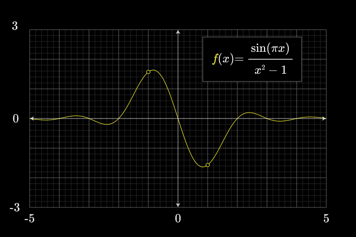
When you plug x=1 into the numerator \sin(\pi x) becomes 0, and similarly the denominator x^{2}-1 also becomes 0, so the function is actually not defined at that input, and the graph should really have a hole there. This also happens at -1, but let's just focus our attention on a single one of these holes for now. Imagine zooming in on the point x=1.

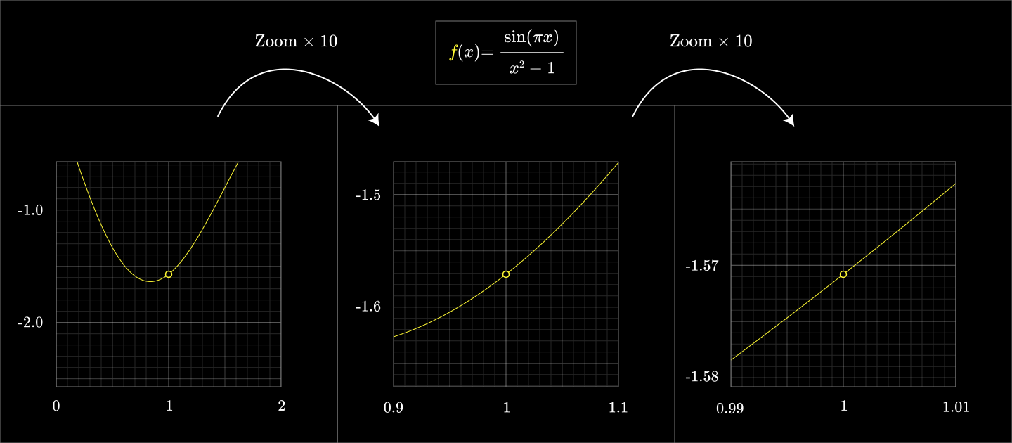
The graph of this function certainly does seem to approach some distinct value at that point, wouldn't you say? So you might ask, how do you figure out what output this approaches as x approaches 1, since you can't just plug in 1?

Well, one way to approximate it would be to plug in a number thats just very very close to 1, like 1.00001. Doing that, you'd find that this should be a number around -1.57. Translating this to the limit notation looks like this:

But is there a way to know precisely what it is? Some systematic process to take an expression like this one, which looks like 0 divided by 0 at some input, and ask what its limit is as x approaches that input? After limits so helpfully let us write the definition for a derivative, derivatives can come back to return the favor and help us evaluate limits. Let me show you what I mean.

Plot numerator and denominator

Let's graph the numerator, \sin(\pi x), and the denominator, x^2-1, of our original function and focus on what's happening at x=1.

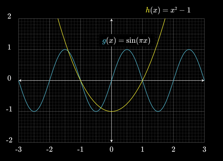
The point here is that \sin(\pi x) and x^2-1 are both 0 at that point, so they cross the x-axis. In the same spirit as plugging in a specific value near 1, like 1.00001, let's zoom in on that point and consider what happens a tiny nudge dx away.

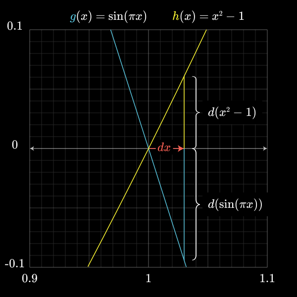
The value of \sin(\pi x) is bumped down by some d(\sin(\pi x)) and the value of x^2-1 is bumped up by some d(x^2-1).

Take a moment to think about how the fraction d(\sin (\pi x)) / d\left(x^{2}-1\right) reframes the initial problem which had previously looked like 0 divided by 0. Why might this lead us towards an exact answer rather than just an approximation?

Since both of these changes are proportional to the small nudge dx, we can go ahead and apply our knowledge of derivatives. Using the chain rule, we know that the change to the function d(\sin(\pi x)) should be around \cos(\pi x) \cdot \pi \cdot dx. Similarly, using the power rule, we know that the change to the function x^2-1 should be around 2 x \cdot dx.

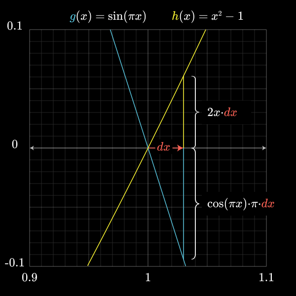
Since we are interested in the fraction of these two functions at the point at x = 1 we can substitute x=1 into both of these expressions and evaluate the fraction.

What this means is that for values of x which are some tiny value dx away from 1, the ratio \sin(\pi x)/(x^2-1) is approximately (-\pi \cdot dx) / (2 \cdot dx). The dx's cancel, so that value is -\pi/2. Importantly, these approximations get more and more accurate for smaller and smaller choices of dx, this ratio -\pi/2 actually tells us the precise limiting value as x approaches 1.

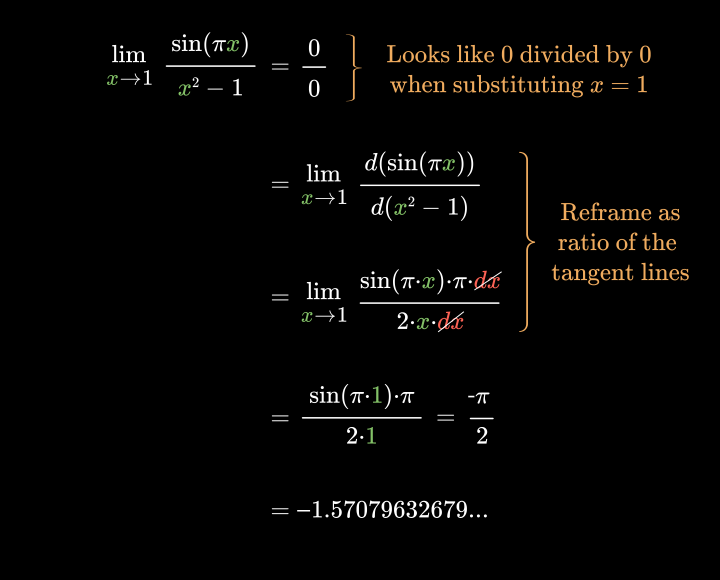
Remember, what that means is that the limiting height on our original graph is evidently exactly -\pi/2.

Generalize

What happened there is a little subtle, so let me show it again, but this time a little more generally. Instead of these two specific functions, which both equal 0 at x=1, think of any two functions f(x) and g(x), which are both 0 at some common value x = a.

The only constraint is that these have to be functions where you're able to take a derivative of them at x = a, meaning they each basically look like a line when you zoom in close enough to that value.

Even though you can't compute f divided by g at this trouble point, since both equal zero, you can ask about this ratio for values of x really really close to a, the limit as x approach a. And it's helpful to think of those nearby inputs as a tiny nudge dx away from a.

The value of f at that nudged point is approximately its derivative, df/dx evaluated at a, times dx. Likewise, the the value of g at that nudged point is approximately the derivative of g, evaluated at a, times dx.

So near this trouble point, the ratio between the outputs of f and g is actually about the same as the derivative of f at a, times dx, divided by the derivative of g at a, times dx. These dx's cancel, so the ratio of f and g near a is about the same as the ratio between their derivatives.

This is a really handy trick for computing a lot of limits. If you come across an expression that seems to equal 0/0 when you plug in some input, just try taking the derivative of the top and bottom expressions, and plugging in that trouble input.

This clever trick is called "L'Hôpital's rule". Interestingly, it was actually discovered by Johann Bernoulli, but L'Hopital was this wealthy dude who essentially paid Bernoulli for the rights to some of his mathematical discoveries. Academia was weird back then, but in a very literal way, it pays to understand these tiny nudges.

Now, you might remember that the definition of a derivative for any given function comes down to computing the limit of a fraction that looks like 0/0, so you might think L'Hopital's rule gives a handy way to discover new derivative formulas. But that would be cheating, since presumably you don't yet know what the derivative on the numerator here is.

When it comes to discovering derivative formulas, something we've been doing a fair amount this series, there is no systematic plug-and-chug method. But that's a good thing. When creativity is needed to solve problems like these, it's a good sign you're doing something real; something that might give you a powerful tool to solve future problems.

In the next lesson, I'll talk about what an integral is, as well as the fundamental theorem of calculus, which is another example of where limits are used to help give a clear meaning to a fairly delicate idea that flirts with infinity.

Exercises