"To many, mathematics is a collection of theorems. For me, mathematics is a collection of examples; a theorem is a statement about a collection of examples and the purpose of proving theorems is to classify and explain the examples."

- John B. Conway

Introduction

When I first learned about Taylor series, I definitely didn't appreciate how important they are. But time and time again they come up in math, physics, and many fields of engineering because they're one of the most powerful tools that math has to offer for approximating functions.

One of the first times this clicked for me as a student was not in a calculus class, but in a physics class. We were studying some problem that had to do with the potential energy of a pendulum, and for that you need an expression for how high the weight of the pendulum is above its lowest point, which works out to be proportional to one minus the cosine of the angle between the pendulum and the vertical.

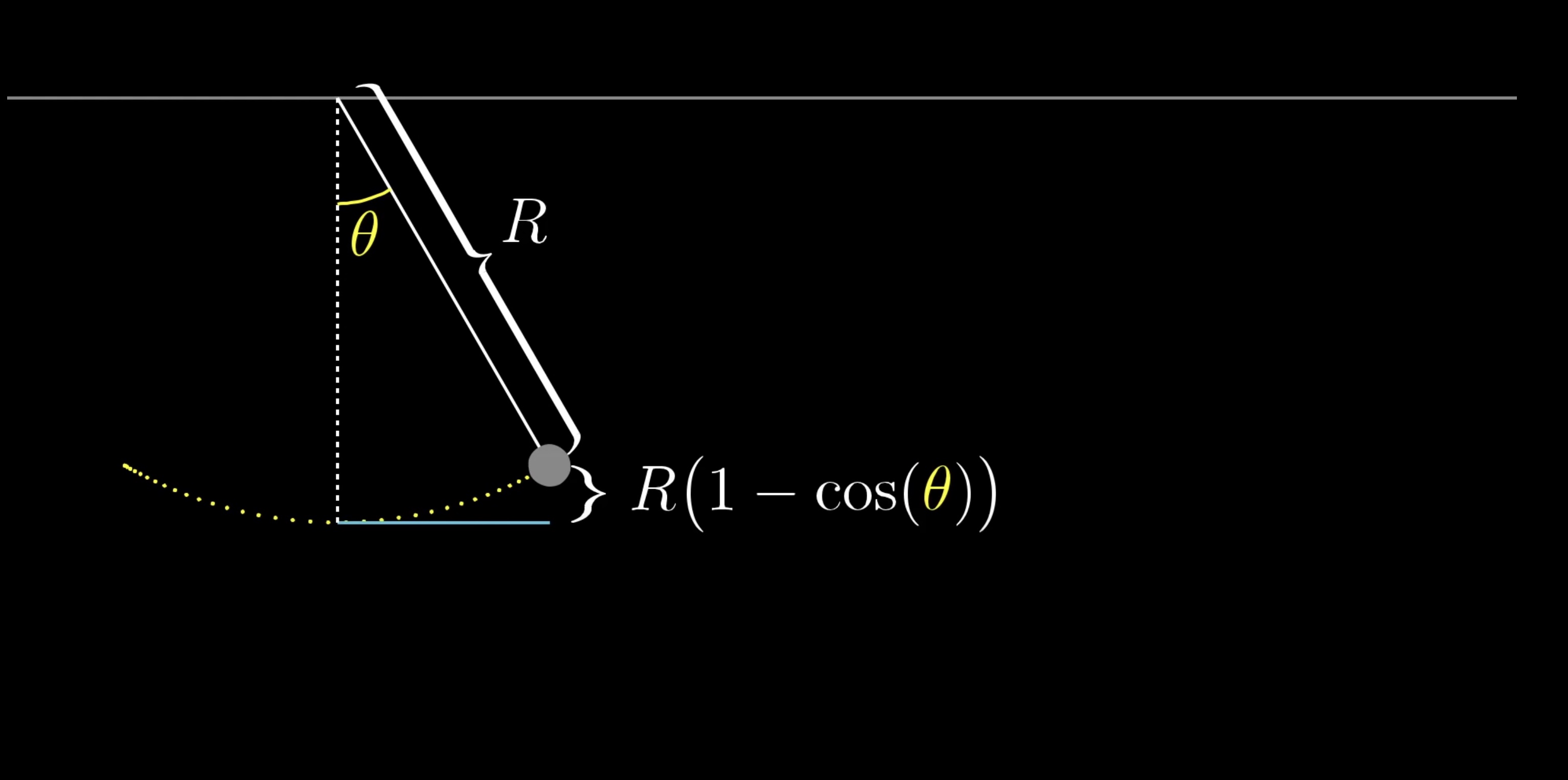
The specifics of the problem we were trying to solve are beyond the point here, but I'll just say that this cosine function made the problem awkward and unwieldy. But by approximating $\cos(\theta)$ as $1 - \frac{\theta^2}{2}$, of all things, everything fell into place much more easily. If you've never seen anything like this before, an approximation like that might seem completely out of left field.

If you graph $\cos(\theta)$ along with this function $1 - \frac{\theta^2}{2}$, they do seem rather close to each other for small angles near 0, but how would you even think to make this approximation? And how would you find this particular quadratic?

The study of Taylor series is largely about taking non-polynomial functions, and finding polynomials that approximate them near some input. The motive is that polynomials tend to be much easier to deal with than other functions: They're easier to compute, easier to take derivatives, easier to integrate... they're just all around friendly.

Approximating $\cos(x)$

Let's look at the function $\cos(x)$, and take a moment to think about how you might find a quadratic approximation near $x = 0$. That is, among all the polynomials that look $c_0 + c_1x + c_2x_2$ for some choice of the constants $c_0$, $c_1$ and $c_2$, find the one that most resembles $\cos(x)$ near $x=0$.

First of all, at the input $0$ the value of $\cos(x)$ is $1$, so if our approximation is going to be any good at all, it should also equal $1$ when you plug in $0$.

Plugging in $0$ just results in whatever $c_0$ is, so we can set that equal to $1$.

This leaves us free to choose constant $c_1$ and $c_2$ to make this approximation as good as we can, but nothing we do to them will change the fact that the output of our approximation at $0$ is equal to $1$.

It would also be good if our approximation had the same tangent slope as $\cos(x)$ at $x=0$. Otherwise, the approximation drifts away from the cosine graph faster than it needs to as $x$ tends away from $0$. The derivative of $\cos(x)$ is $-\sin(x)$, and at $x=0$ that equals $0$, meaning its tangent line is flat.

This is the same as making the derivative of our approximation as close as we can to the derivative of our original function $\cos(x)$.

Setting $c_1$ equal to $0$ ensures that our approximation matches the tangent slope of $\cos(x)$ at this point.

This is the same approximation we just had! But we should feel confident that the process is working, because our approximation now equals the value and slope of $\cos(x)$ a $x=0$, leaving us free to change $c_2$.

We can take advantage of the fact that the cosine graph curves downward above $x=0$, it has a negative second derivative. Or in other words, even though the rate of change is $0$ at that point, the rate of change itself is decreasing around that point.

Specifically, since its derivative is $-\sin(x)$ its second derivative is $-\cos(x)$, so at $x=0$ its second derivative is $-1$.

Just as we wanted the derivative of our approximation to match that of cosine, we'll also make sure that their second derivatives match so as to ensure that they curve at the same rate. The slope of our polynomial shouldn't drift away from the slope of $\cos(x)$ any more quickly than it needs to.

We can compute that at $x=0$, the second derivative of our polynomial is $2c_2$. In fact, that's its second derivative everywhere, it is a constant. To make sure this second derivative matches that of $\cos(x)$, we want it to equal $-1$, which means $c_2 = -\frac{1}{2}$. This locks in a final value for our approximation:

To get a feel for how good this is, let's try it out for $x = 0.1$

That's pretty good!

Take a moment to reflect on what just happened. You had three degrees of freedom with a quadratic approximation, the coefficients in the expression $c_0 + c_1 x + c_2 x^2$.

• $c_0$ was responsible for making sure that the output of the approximation matches that of $\cos(x)$ at $x=0$.
• $c_1$ was in charge of making sure the derivatives match at that point.
• $c_2$ was responsible for making sure the second derivatives match up.

This ensures that the way your approximation changes as you move away from $x=0$, and the way that the rate of change itself changes, is as similar as possible to behavior of $\cos(x)$, given the amount of control you have.

Better Approximations

You could give yourself more control by allowing more terms in your polynomial and matching higher-order derivatives of $\cos(x)$. For example, let's say we add on the term $c_3 x^3$ for some constant $c_3$.

If you take the third derivative of a cubic polynomial, anything quadratic or smaller goes to $0$. As for that last term, after three iterations of the power rule it looks like $1 \cdot 2 \cdot 3 \cdot c_3$.

On the other hand, the third derivative of $\cos(x)$ is $\sin(x)$, which equals $0$ at $x=0$, so to make the third derivatives match, the constant $c_3$ should be $0$.

In other words, not only is $1 - \frac{1}{2}x^2$ the best possible quadratic approximation of $\cos(x)$ around $x=0$, it's also the best possible cubic approximation.

You can actually make an improvement by adding a fourth order term, $c_4x^4$. The fourth derivative of $\cos(x)$ is also $\cos(x)$, which equals $1$ at $x=0$. And what's the fourth derivative of our polynomial with this new term?

When you keep applying the power rule over and over, with those exponents all hopping down to the front, you end up with $1 \cdot 2 \cdot 3 \cdot 4 \cdot c_4$, which is $24c_4$.

So if we want this to match the fourth derivative of $\cos(x)$, which at $x=0$ is $1$, then we must set $c_4 = \frac{1}{24}$.

This polynomial $1 - \frac{1}{2}x^2 + \frac{1}{24}x^4$ is a very close approximation for $\cos(x)$ around $x = 0$ and for any physics problem involving the cosine of some small angle, for example, predictions would be almost unnoticeably different if you substituted this polynomial for $\cos(x)$.

Generalizing

It's worth stepping back to notice a few things about this process. First, factorial terms naturally come up in this process. When you take $n$ derivatives of $x_n$, letting the power rule just keep cascading, what you're left with is $1 \cdot 2 \cdot 3$ and on up to $n$.

So you don't simply set the coefficients of the polynomial equal to whatever derivative value you want, you have to divide by the appropriate factorial to cancel out this effect. For example, in the approximation for $\cos(x)$, the $x_4$ coefficient is the fourth derivative of cosine, $1$, divided by $4! = 24$.

The second thing to notice is that adding new terms, like this $c_4x^4$, doesn't mess up what old terms should be, and that's important. For example, the second derivative of this polynomial at $x = 0$ is still equal to $2$ times the second coefficient, even after introducing higher order terms to the polynomial.

This is because we're plugging in $x=0$, so the second derivative of any higher order terms, which all include an $x$, will wash away. The same goes for any other derivative, which is why each derivative of a polynomial at $x=0$ is controlled by one and only one coefficient.

Comprehension Question

Just like $\cos(x)$, the function $\sin(x)$ is a situtation where we know its derivative and its value at $x=0$. Let's apply the same process to find the third degree taylor polynomial of $\sin(x)$.

Approximating around other points

If instead, you were approximating near an input other than $0$, like $x=\pi$, to get the same effect you would have to write your polynomial in terms of powers of $(x - \pi)$. Or more generally, powers of $(x - a)$ for some constant $a$.

This makes it look notably more complicated, but it's all to make sure plugging in $x=\pi$ results in a lot of nice cancelation so that the value of each higher-order derivative is controlled by one and only one coefficient.

Finally, on a more philosophical level, notice how we're taking information about the higher-order derivatives of a function at a single point, and translating it into information (or at least approximate information) about the value of that function near that point. This is the major takeaway for Taylor series: Differential information about a function at one value tells you something about an entire neighborhood around that value.

We can take as many derivatives of $\cos(x)$ as we want, it follows this nice cyclic pattern $\cos(x)$, $-\sin(x)$, $-\cos(x)$, $\sin(x)$, and repeat.

So the value of these derivative of $x=0$ have the cyclic pattern $1$, $0$, $-1$, $0$, and repeat. And knowing the values of all those higher-order derivatives is a lot of information about $\cos(x)$, even though it only involved plugging in a single input, $x=0$.

That information is leveraged to get an approximation around this input by creating a polynomial whose higher order derivatives, match up with those of $\cos(x)$, following this same $1$, $0$, $-1$, $0$ cyclic pattern.

To do that, make each coefficient of this polynomial follow this same pattern, but divide each one by the appropriate factorial which cancels out the cascading effects of many power rule applications. The polynomials you get by stopping this process at any point are called "Taylor polynomials" for $\cos(x)$.

Other Functions

More generally, if we were dealing with some function other than cosine, you would compute its derivative, second derivative, and so on, getting as many terms as you'd like, and you'd evaluate each one at $x=0$.

Then for your polynomial approximation, the coefficient of each $x^n$ term should be the value of the $n$-th derivative of the function at $0$, divided by $(n!)$.

When you see this, think to yourself that the constant term ensures that the value of the polynomial matches that of $f(x)$ at $x=0$, the next term ensures that the slope of the polynomial matches that of the function, the next term ensure the rate at which that slope changes is the same, and so on, depending on how many terms you want.

The more terms you choose, the closer the approximation, but the tradeoff is that your polynomial is more complicated. And if you want to approximate near some input $a$ other than $0$, you write the polynomial in terms of $(x-a)$ instead, and evaluate all the derivatives of $f$ at that input $a$.

This is what Taylor series look like in their fullest generality. Changing the value of $a$ changes where the approximation is hugging the original function; where its higher order derivatives will be equal to those of the original function.

A meaningful example

One of the simplest meaningful examples is to approximate the function $f(x) = e^x$, around the input $x=0$. Computing its derivatives is nice since the derivative of $e^x$ is also $e^x$, so its second derivative is also $e^x$, as is its third, and so on.

So at the point $x=0$, all of the derivatives are equal to $1$. This means our polynomial approximation looks like $(1) + (1)x + (1)\frac{x^2}{2!} + (1)\frac{x^3}{3!} + (1)\frac{x^4}{4!}$, and so on, depending on how many terms you want. These are the Taylor polynomials for $e^x$.

Infinity and convergence

We could call it an end here, and you'd have you'd have a phenomenally useful tool for approximations with these Taylor polynomials. But if you're thinking like a mathematician, one question you might ask is if it makes sense to never stop, and add up infinitely many terms.

In math, an infinite sum is called a "series", so even though one of the approximations with finitely many terms is called a "Taylor polynomial" for your function, adding all infinitely many terms gives what's called a "Taylor series".

You have to be careful with the idea of an infinite sum because one can never truly add infinitely many things; you can only hit the plus button on the calculator so many times. The more precise way to think about a series is to ask what happens as you add more and more terms. If the partial sums you get by adding more terms one at a time approach some specific value, you say the series converges to that value.

It's a mouthful to always say "The partial sums of the series converge to such and such value", so instead mathematicians often think about it more compactly by extending the definition of equality to include this kind of series convergence. That is, you'd say this infinite sum equals the value its partial sums converge to.

For example, look at the Taylor polynomials for $e^x$, and plug in some input like $x = 1$.

As you add more and more polynomial terms, the total sum gets closer and closer to the value $e$. The precise-but-verbose way to say this is "the partial sums of the series on the right converge to $e$." More briefly, most people would abbreviate this by simply saying "the series equals $e$."

In fact, it turns out that if you plug in any other value of $x$, like $x=2$, and look at the value of higher and higher order Taylor polynomials at this value, they will converge towards $e^x$, in this case $e^2$.

This is true for any input, no matter how far away from $0$ it is, even though these Taylor polynomials are constructed only from derivative information gathered at the input $0$. In a case like this, we say $e^x$ equals its Taylor series at all inputs $x$. This is a somewhat magical fact! It means all of the information about the function is somehow captured purely by higher-order derivatives at a single input, namely $x=0$.

Limitations for $\ln(x)$

Although this is also true for some other important functions, like sine and cosine, sometimes these series only converge within a certain range around the input whose derivative information you're using. If you work out the Taylor series for $\ln(x)$ around the input $x = 1$, which is built from evaluating the higher order derivatives of $\ln(x)$ at $x=1$, this is what it looks like.

When you plug in an input between $0$ and $2$, adding more and more terms of this series will indeed get you closer and closer to the natural log of that input.

But outside that range, even by just a bit, the series fails to approach anything. As you add more and more terms the sum bounces back and forth wildly. The partial sums do not approach the natural log of that value, even though the $\ln(x)$ is perfectly well defined for $x > 2$.

In some sense, the derivative information of $\ln(x)$ at $x=1$ doesn't propagate out that far. In a case like this, where adding more terms of the series doesn't approach anything, you say the series diverges.

That maximum distance between the input you're approximating near, and points where the outputs of these polynomials actually do converge, is called the "radius of convergence" for the Taylor series.

Summary

There remains more to learn about Taylor series, their many use cases, tactics for placing bounds on the error of these approximations, tests for understanding when these series do and don't converge. For that matter there remains more to learn about calculus as a whole, and the countless topics not touched by this series.

The goal with these videos is to give you the fundamental intuitions that make you feel confident and efficient learning more on your own, and potentially even rediscovering more of the topic for yourself. In the case of Taylor series, the fundamental intuition to keep in mind as you explore more is that they translate derivative information at a single point to approximation information around that point.