Backpropagation calculus
The math of backpropagation, the algorithm by which neural networks learn.
The hard assumption here is that you've read , giving an intuitive walkthrough of the backpropagation algorithm. Here, we get a bit more formal and dive into the relevant calculus. It's normal for this to be a little confusing, so be sure to pause and ponder throughout.
As a quick reminder, backpropagation is an algorithm for calculating the gradient of the cost function of a network.
\textcolor{red}{\nabla C} =
\left[\begin{array}{c}
\frac{\textcolor{red}{\partial C}}{\textcolor{blue}{\partial w^{(1)}}} \\[0.8em]
\frac{\textcolor{red}{\partial C}}{\textcolor{pink}{\partial b^{(1)}}} \\[0.5em]
\vdots \\[0.5em]
\frac{\textcolor{red}{\partial C}}{\textcolor{blue}{\partial w^{(L)}}} \\[0.8em]
\frac{\textcolor{red}{\partial C}}{\textcolor{pink}{\partial b^{(L)}}}
\end{array}\right]
The entries of the gradient vector are the partial derivatives of the cost function with respect to all the different weights and biases of the network, so it's really those derivatives that backpropagation helps us find.
In the last lesson we talked about the intuitive feeling you might have for how backpropagation works, so now our focus will be on connecting that intuition with the appropriate calculus.
(For those uncomfortable with the relevant calculus, I do have a whole series on the topic.)
The main goal here is to show how people in machine learning commonly think about the in the context of networks, which can feel a bit different than how most introductory calculus courses approach the subject.
Calculating the Gradient with Backpropagation
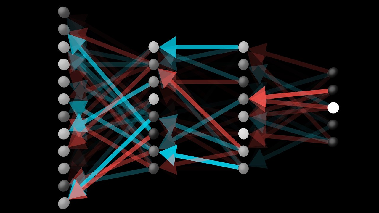
Let's start with an extremely simple network, where each layer has just one neuron.

We'll start with a very simple neural network.
This network is determined by 3 weights (one for each connection) and 3 biases (one for each neuron, except the first), and our goal is to understand how changing each of them will affect the cost function. That way we know which adjustments will cause the most efficient decrease to the cost.

How strongly do these six weights and biases affect the value of the cost function?
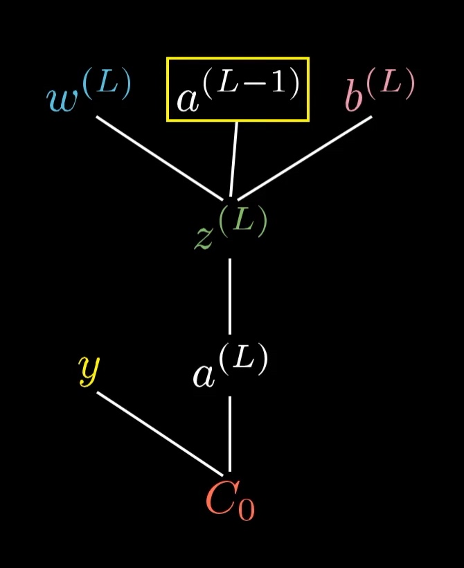
For now, let's just focus on the connection between the last two neurons. I'll label the activation of that last neuron with a superscript L, indicating which layer it's in, so the activation of the previous neuron is a^{(L-1)}:
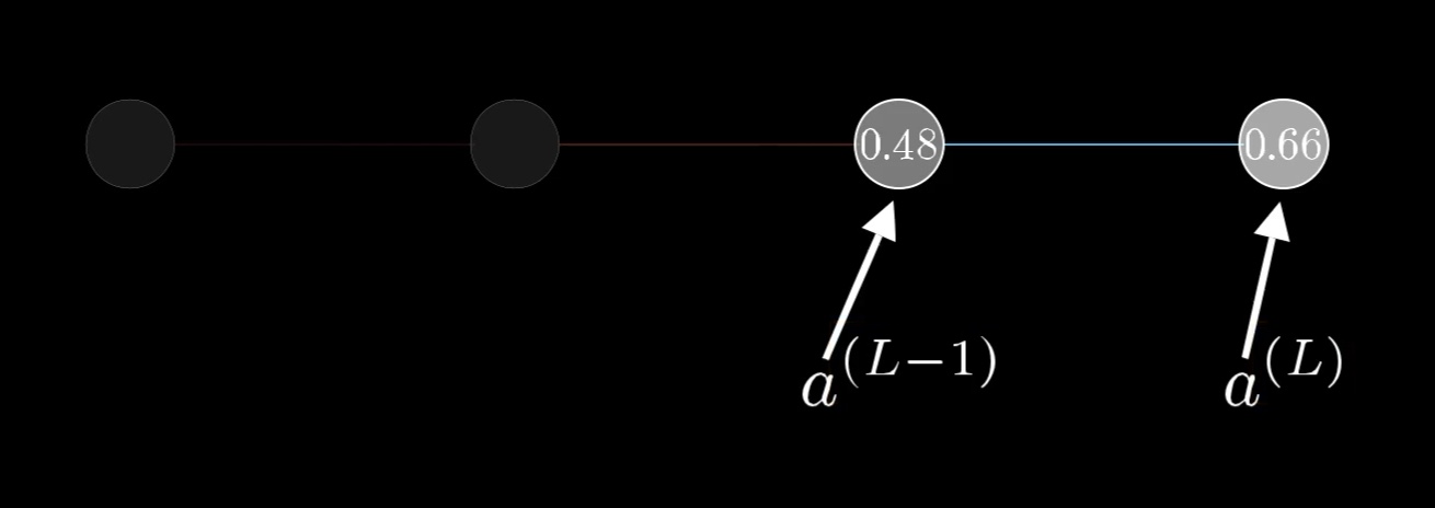
We label the activations of the neurons based on which layer they're in, where
L is the last layer of the network.
To be clear, these are not exponents. They are just ways of indexing what layer we're talking about, since we want to save subscripts for different indices later on.
Let's say that for a certain training example, the desired output is \textcolor{gold}{y}. That means that the cost for this one training example is \textcolor{red}{C_0} = (a^{(L)} - \textcolor{gold}{y})^2.

The cost to the network for this one training example is just the difference between the actual output and the desired output squared.
As a reminder, this last activation a^{(L)} is determined by a weight, a bias, and the previous neuron's activation, all pumped through some special nonlinear function like a sigmoid or a ReLU.
a^{(L)} = \sigma\left(\textcolor{blue}{w^{(L)}} a^{(L-1)} + \textcolor{pink}{b^{(L)}}\right)It'll make things easier for us to give a special name to this weighted sum, like \textcolor{green}{z}, with the same superscript as the activation:
\begin{align*}
\textcolor{green}{z^{(L)}} &= \textcolor{blue}{w^{(L)}} a^{(L-1)} + \textcolor{pink}{b^{(L)}} \\
a^{(L)} &= \sigma\left(\textcolor{green}{z^{(L)}}\right)
\end{align*}
A way you might conceptualize this is that the weight, the previous activation, and the bias together let us compute \textcolor{green}{z^{(L)}}, which in turn lets us compute a^{(L)}, which in turn, along with the constant \textcolor{gold}{y}, lets us compute the cost.
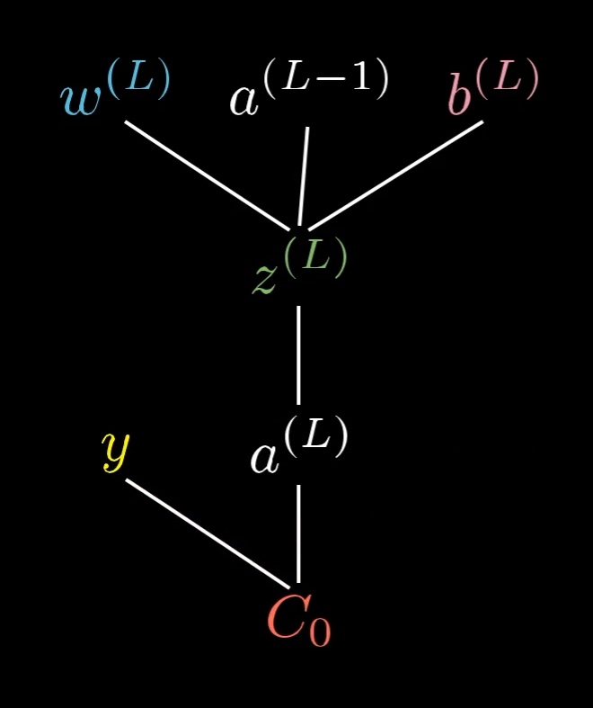
This tree shows which values depend on which other values in our network.
And of course, a^{(L-1)} is influenced by its own weight and bias, which means our tree actually extends up higher...
...but we won't focus on that right now.
All of these are just numbers, so it can be nice to think of each variable as having its own little number line.
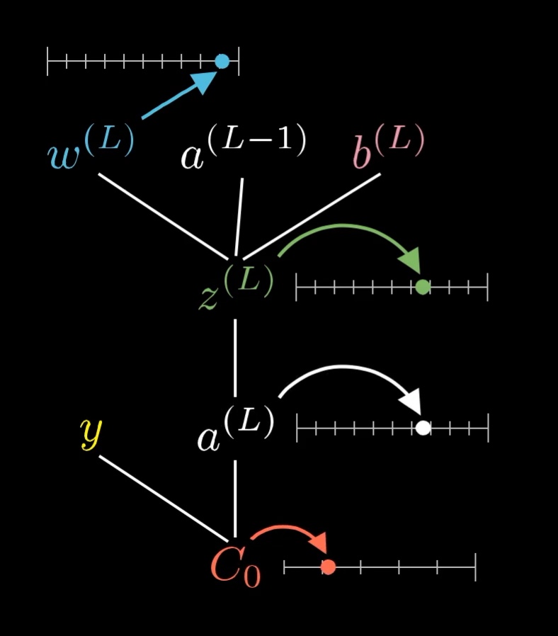
Each of these variables has a value that we can place on its own little number line.
Computing The First Derivative
Our first goal is to understand how sensitive the cost \textcolor{red}{C_0} is to small changes in the weight \textcolor{blue}{w^{(L)}}. That is, we want to know the derivative \frac{\textcolor{red}{\partial C_0}}{\textcolor{blue}{\partial w^{(L)}}}.
When you see this \textcolor{blue}{\partial w^{(L)}} term, think of it as meaning "some tiny nudge to \textcolor{blue}{w^{(L)}}", like a change by 0.01. And think of this \textcolor{red}{\partial C_0} term as meaning "whatever the resulting nudge to the cost is." We want their ratio.
Conceptually, this tiny nudge to \textcolor{blue}{w^{(L)}} causes some nudge to \textcolor{green}{z^{(L)}}, which in turn causes some change to a^{(L)}, which directly influences the cost, \textcolor{red}{C_0}.

The nudge to \textcolor{blue}{w^{(L)}} has a chain of effects which eventually causes a nudge to \textcolor{red}{C_0}.
So we break this up by first taking the ratio of a tiny change to \textcolor{green}{z^{(L)}} to the tiny change in \textcolor{blue}{w^{(L)}}. That is, the derivative of \textcolor{green}{z^{(L)}} with respect to \textcolor{blue}{w^{(L)}}. Likewise, consider the ratio of a tiny change to a^{(L)} to the tiny change in \textcolor{green}{z^{(L)}} that caused it, as well as the ratio between the final nudge to \textcolor{red}{C_0} and this intermediate nudge to a^{(L)}.

This is the , where multiplying these three ratios gives us the sensitivity of \textcolor{red}{C_0} to small changes in \textcolor{blue}{w^{(L)}}.
The Constituent Derivatives
We've broken down the derivative we actually want, \frac{\textcolor{red}{\partial C_0}}{\textcolor{blue}{\partial w^{(L)}}}, into its constituent parts. Now we just need to compute the values of the three individual derivatives that make it up.
To compute each derivative, we'll use some relevant formula from the way we've defined our neural network.
\begin{align*}

\textcolor{green}{z^{(L)}} &= \textcolor{blue}{w^{(L)}} a^{(L-1)} + \textcolor{pink}{b^{(L)}}
\quad &\longrightarrow \quad
\frac{\textcolor{green}{\partial z^{(L)}}}{\textcolor{blue}{\partial w^{(L)}}} &= a^{(L-1)} \\ \\

a^{(L)} &= \sigma\left(\textcolor{green}{z^{(L)}}\right)
\quad &\longrightarrow \quad
\frac{\partial a^{(L)}}{\textcolor{green}{\partial z^{(L)}}} &= \sigma^{\prime}\left(\textcolor{green}{z^{(L)}}\right) \\ \\

\textcolor{red}{C_0} &= \left(a^{(L)} - \textcolor{gold}{y}\right)^{2}
\quad &\longrightarrow \quad
\frac{\textcolor{red}{\partial C_0}}{\partial a^{(L)}} &= 2\left(a^{(L)} - \textcolor{gold}{y}\right)

\end{align*}
As you can see, each derivative is pretty straightforward once you know which equation to start from.
It's worth taking a moment to reflect on what these expressions actually mean. Notice the first derivative we computed, \frac{\textcolor{green}{\partial z^{(L)}}}{\textcolor{blue}{\partial w^{(L)}}}. It's telling us that changing the weight has a stronger effect on \textcolor{green}{z^{(L)}} (and therefore a stronger effect on the cost) when the previous neuron is more active. This is where that biological idea that "neurons that fire together, wire together" is mirrored in our math.
Also pay attention to the final derivative, \frac{\textcolor{red}{\partial C_0}}{\partial a^{(L)}}. It's proportional to the difference between the actual output and the desired output. This means that when the actual output is way different than what we want it to be, even small nudges to the activation stand to make a big difference to the cost.
Putting It All Together
We originally broke down \frac{\textcolor{red}{\partial C_{0}}}{\textcolor{blue}{\partial w^{(L)}}} into three separate derivatives using the chain rule:
\frac{\textcolor{red}{\partial C_{0}}}{\textcolor{blue}{\partial w^{(L)}}} =
\frac{\textcolor{green}{\partial z^{(L)}}}{\textcolor{blue}{\partial w^{(L)}}}
\frac{\partial a^{(L)}}{\textcolor{green}{\partial z^{(L)}}}
\frac{\textcolor{red}{\partial C_0}}{\partial a^{(L)}}
Putting this together with our constituent derivatives, we get:
\frac{\textcolor{red}{\partial C_{0}}}{\textcolor{blue}{\partial w^{(L)}}} =
a^{(L-1)} \sigma^{\prime}\left(\textcolor{green}{z^{(L)}}\right) 2\left(a^{(L)} - \textcolor{gold}{y}\right)
This formula tells us how a nudge to that one particular weight in the last layer will affect the cost for that one particular training example. This is just one very specific piece of information, and we'll need to calculate a lot more to get the entire gradient vector.
But the good news is that we've already laid the foundations for the rest of the work that needs to be done. Now it's just a process of generalizing our results until we have an understanding (in the form of the gradient vector) of how all the weights and biases in the network affect the overall cost.
The Cost for All Training Data
Notice the little subscript zero in the derivative we calculated, \frac{\textcolor{red}{\partial C_{0}}}{\textcolor{blue}{\partial w^{(L)}}}. That's there because \textcolor{red}{C_0} is just the cost of a single training example.
The full cost function for the network (\textcolor{red}{C}) is the average all the individual costs for each training example:
\textcolor{red}{C} = \frac{1}{n} \sum_{k=0}^{n-1} \textcolor{red}{C_k}So if we want the derivative of \textcolor{red}{C} with respect to the weight (rather than the derivative of \textcolor{red}{C_0} with respect to the weight), we need to take the average of all the individual derivatives:
\frac{\textcolor{red}{\partial C}}{\textcolor{blue}{\partial w^{(L)}}} =
\frac{1}{n} \sum_{k=0}^{n-1} \frac{\textcolor{red}{\partial C_k}}{\textcolor{blue}{\partial w^{(L)}}}
This expression tells us how the overall cost of the network will change when we wiggle the last weight.
Recall that the entries of the gradient vector are the partial derivatives of the cost function \textcolor{red}{C} with respect to every weight and bias in the network. So this derivative, \frac{\textcolor{red}{\partial C}}{\textcolor{blue}{\partial w^{(L)}}}, is one of its entries!
The Derivative for All Weights And Biases
But to compute the full gradient, we will also need all the other derivatives with respect to all the other weights and biases in the entire network.
\textcolor{red}{\nabla C} =
\left[\begin{array}{c}
\frac{\textcolor{red}{\partial C}}{\textcolor{blue}{\partial w^{(1)}}} \\[0.8em]
\frac{\textcolor{red}{\partial C}}{\textcolor{pink}{\partial b^{(1)}}} \\[0.5em]
\vdots \\[0.5em]
\frac{\textcolor{red}{\partial C}}{\textcolor{blue}{\partial w^{(L)}}} \\[0.8em]
\frac{\textcolor{red}{\partial C}}{\textcolor{pink}{\partial b^{(L)}}}
\end{array}\right]
Let's work on computing the bias in the last layer next.
The Bias
The good news is that the sensitivity of the cost function to a change in the bias is almost identical to the equation for a change to the weight.
As a reminder, here's the equation we found earlier for the derivative with respect to the weight in the last layer:
\frac{\textcolor{red}{\partial C_{0}}}{\textcolor{blue}{\partial w^{(L)}}} =
\frac{\textcolor{green}{\partial z^{(L)}}}{\textcolor{blue}{\partial w^{(L)}}}
\frac{\partial a^{(L)}}{\textcolor{green}{\partial z^{(L)}}}
\frac{\textcolor{red}{\partial C_0}}{\partial a^{(L)}}
And here's the new equation for the derivative with respect to the bias in the last layer (instead of the weight):
\frac{\textcolor{red}{\partial C_{0}}}{\textcolor{pink}{\partial b^{(L)}}} =
\frac{\textcolor{green}{\partial z^{(L)}}}{\textcolor{pink}{\partial b^{(L)}}}
\frac{\partial a^{(L)}}{\textcolor{green}{\partial z^{(L)}}}
\frac{\textcolor{red}{\partial C_0}}{\partial a^{(L)}}
All we've done is replaced the \frac{\textcolor{green}{\partial z^{(L)}}}{\textcolor{blue}{\partial w^{(L)}}} with a \frac{\textcolor{green}{\partial z^{(L)}}}{\textcolor{pink}{\partial b^{(L)}}}.
Luckily, this new derivative is simply 1:
\textcolor{green}{z^{(L)}} = \textcolor{blue}{w^{(L)}} a^{(L-1)} + \textcolor{pink}{b^{(L)}}
\quad \longrightarrow \quad
\frac{\textcolor{green}{\partial z^{(L)}}}{\textcolor{pink}{\partial b^{(L)}}} = 1
So the derivative for the bias turns out to be even simpler than the derivative for the weight.
That's two gradient entries taken care of.
Previous Layers' Weights and Biases
We've now determined how changes to the last weight and last bias in our super-simple neural network will affect the overall cost, which means we already have two of the entries of our gradient vector.
All the other weights and biases lie in earlier layers of the network, meaning their influence on the cost is less direct. The way we handle them is to first see how sensitive the cost is to the value of that neuron in the second-to-last layer, a^{(L - 1)}, and then to see how sensitive that value is to all the preceding weights and biases.
We still need to figure out what to do with the activation of the neuron in the previous layer.
Unsurprisingly, the derivative of the cost with respect to that activation looks very similar to what we've seen already:
\frac{\textcolor{red}{\partial C_{0}}}{\partial a^{(L-1)}} =
\frac{\textcolor{green}{\partial z^{(L)}}}{\partial a^{(L-1)}}
\frac{\partial a^{(L)}}{\textcolor{green}{\partial z^{(L)}}}
\frac{\textcolor{red}{\partial C_0}}{\partial a^{(L)}}
To solve it, we just need to figure out the value of \frac{\textcolor{green}{\partial z^{(L)}}}{\partial a^{(L-1)}}, which we can do by reminding ourselves of the definition of \textcolor{green}{z^{(L)}}.
\textcolor{green}{z^{(L)}} = \textcolor{blue}{w^{(L)}} a^{(L-1)} + \textcolor{pink}{b^{(L)}}
\quad \longrightarrow \quad
\frac{\textcolor{green}{\partial z^{(L)}}}{\partial a^{(L-1)}} = \textcolor{blue}{w^{(L)}}
So when the activation in the second-to-last layer is changed, the effect on \textcolor{green}{z^{(L)}} will be proportional to the weight.
But we don't really care about what happens when we change the activation directly, because we don't have control over that. All we can change, when trying to improve the network through gradient descent, is the values of the weights and biases.
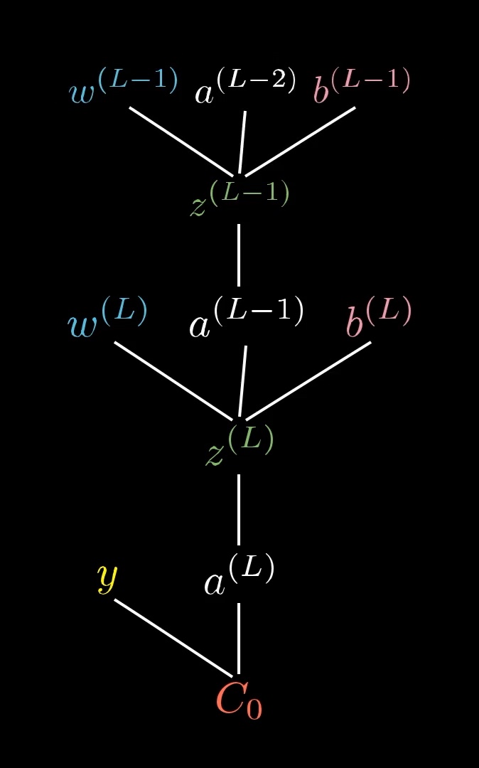
The trick here is to remember that the activation in the previous layer is actually determined by its own set of weights and biases. In reality, our tree stretches back farther than we've shown so far:
The activation in the second-to-last layer is determined by its own weights and biases. The plot thickens.
This is where the propagation backwards comes in. Even though we won't be able to directly change that activation, it's helpful to keep track of, because we can just keep iterating this chain rule backwards to see how sensitive the cost function is to previous weights and biases.
For example, there is a long chain of dependencies between the weight \textcolor{blue}{w^{(L - 1)}} and the cost \textcolor{red}{C_0}. The way this will show up mathematically is that the partial derivative of the cost with respect to that weight will look like a long chain of partial derivatives for each intermediate step.
How would you break down the derivative \frac{\textcolor{red}{\partial C_0}}{\textcolor{blue}{\partial w^{(L-1)}}} into bite-size steps using the chain rule? Take a moment to trace it out. (It might be helpful to refer back to the extended tree image above.)
By tracking the dependencies through our tree, and multiplying together a long series of partial derivatives, we can now calculate the derivative of the cost function with respect to any weight or bias in the entire network. We're simply applying the same chain rule idea we've been using all along!
And since we can get any derivative we want, we can compute the entire gradient vector. Job done! At least for this network.
More Complicated Networks
So that's how you get the relevant derivatives for this super simple network.
You might think that this is an overly simple example, because each layer has just one neuron, and that it's going to get dramatically more complicated for a real network. But honestly, not that much changes when we give the layers multiple neurons; it's just a few more indices to keep track of really.
Rather than the activation in a given layer simply being a^{(L)}, it will also have a subscript indicating which neuron of the layer it is.
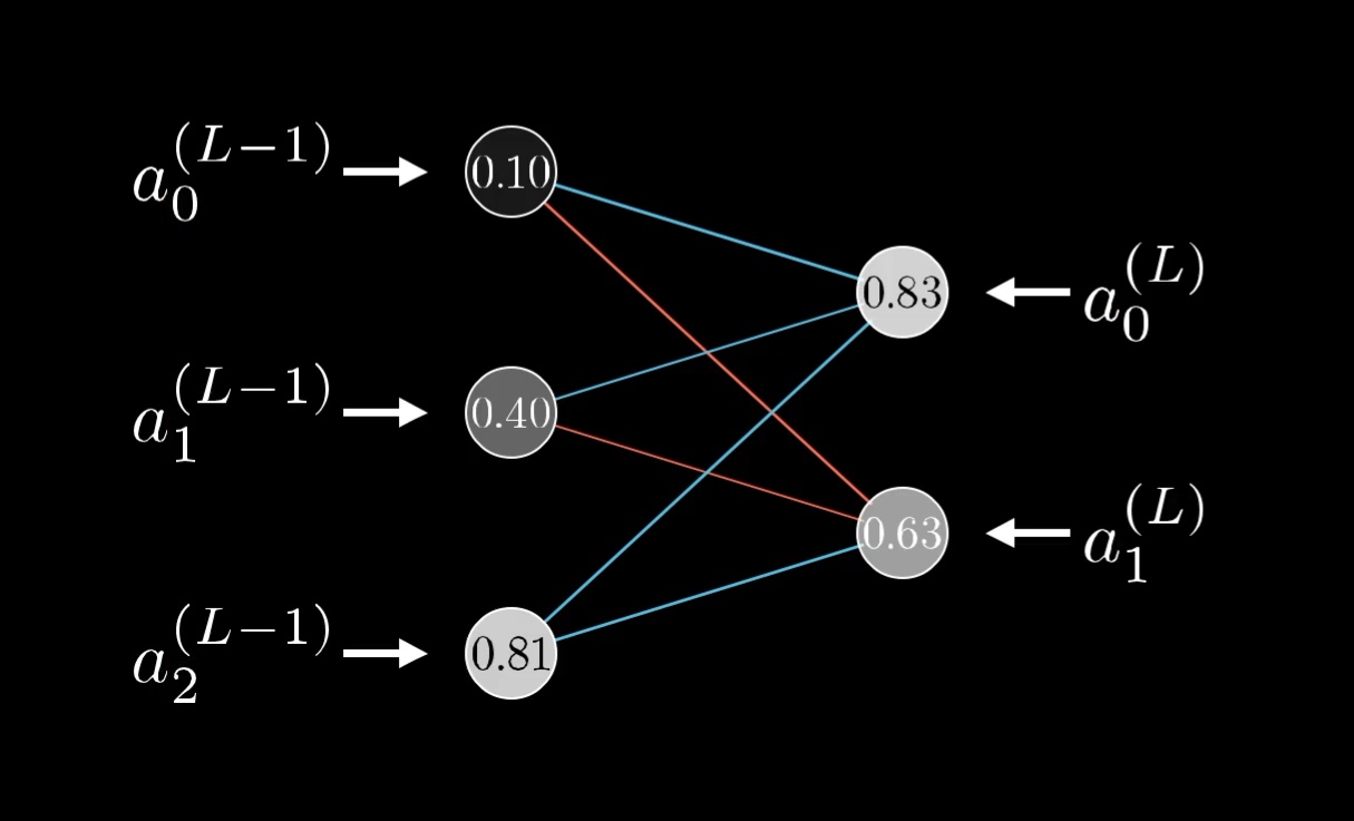
The superscript on each neuron indicates which layer it's on, and the subscript indicates which neuron it is.
Let's use the letter k to index the layer (L-1), and j to index the layer (L).

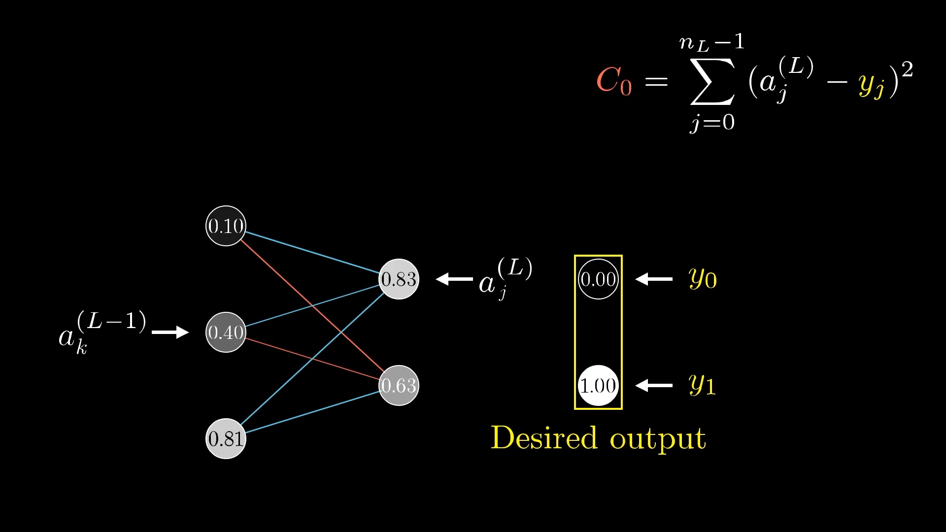
For the cost, again look at what the desired output is, then add up the squares of the differences between these last layer activations and this desired output. That is, sum over (a^{(L)}_j - \textcolor{gold}{y_j})^2.
Each weight now needs a few more indices to keep track of where it is, so let's call the weight of the edge connecting this kth neuron to this jth neuron \textcolor{blue}{w^{(L)}_{jk}}:
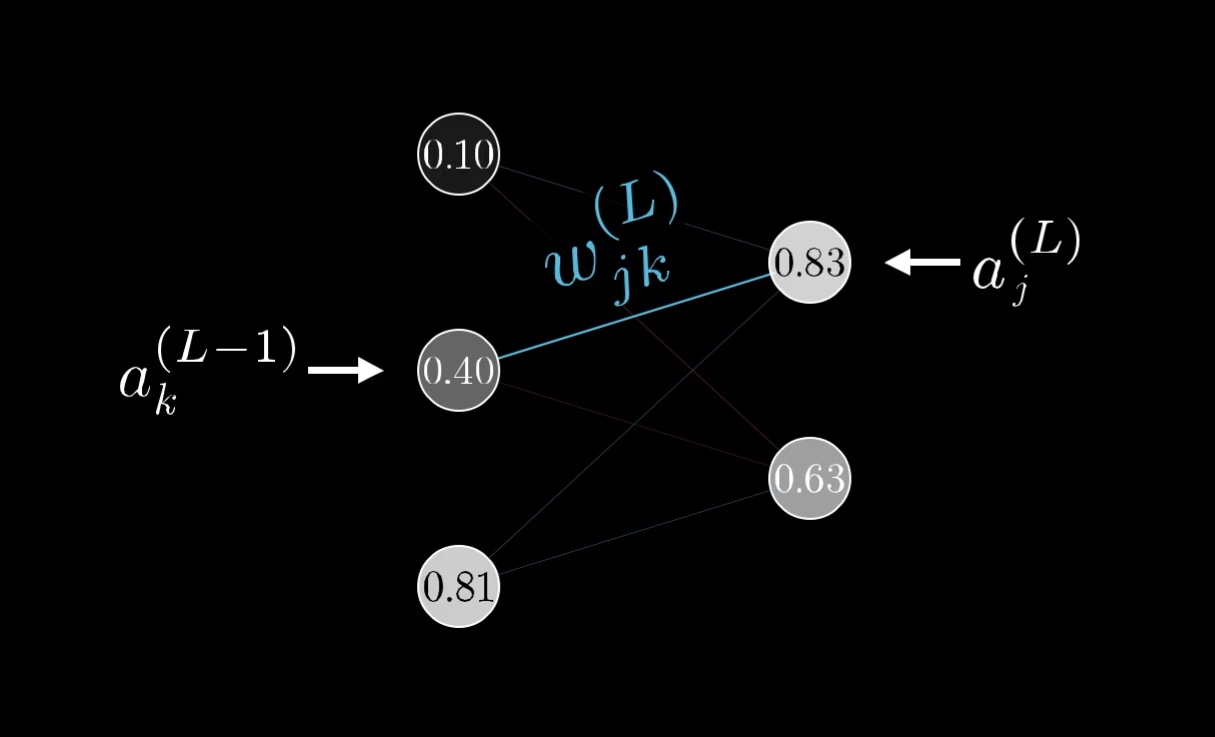
Those indices, \textcolor{blue}{jk}, might feel backwards at first, but it lines up with how you'd index the weight matrix I talked about in .
It's still nice to give a name to the relevant weighted sum, like \textcolor{green}{z}.
\textcolor{green}{z_j^{(L)}} =

\textcolor{blue}{w_{j0}^{(L)}} a_0^{(L-1)} +
\textcolor{blue}{w_{j1}^{(L)}} a_1^{(L-1)} +
\textcolor{blue}{w_{j2}^{(L)}} a_2^{(L-1)} +
\textcolor{pink}{b_j^{(L)}}
We still wrap this weighted sum with a special function like a sigmoid or a ReLU to get the final activation.
The new equations we have are all essentially the same as what we had in the one-neuron-per-layer case. Indeed, the chain-rule derivative expression describing how sensitive the cost is to a particular weight is essentially identical to what we had before.
\frac{\textcolor{red}{\partial C_0}}{\textcolor{blue}{\partial w_{jk}^{(L)}}} =

\frac{\textcolor{green}{\partial z_j^{(L)}}}{\textcolor{blue}{\partial w_{jk}^{(L)}}}
\frac{\partial a_j^{(L)}}{\textcolor{green}{\partial z_j^{(L)}}}
\frac{\textcolor{red}{\partial C_0}}{\partial a_j^{(L)}}
The only difference is that we're keeping track of more indices, j and k, which tell us which weight specifically we're talking about. After all, there are now many weights connecting the second-to-last layer to the last.
What does change, though, is the derivative of the cost with respect to one of the activations in the layer (L-1), \frac{\textcolor{red}{\partial C_0}}{\partial a_k^{(L-1)}}.
This neuron influences the cost function through multiple paths.
So to understand the sensitivity of the cost function to this neuron, you have to add up the influences along each of those different paths. That is, on the one hand, it influences a^{(L)}_0, which plays a role in the cost function, but on the other hand it influences a^{(L)}_1, which also plays a role in the cost function.
Because this previous-layer neuron influences the cost along multiple different paths, the derivative of the cost with respect to this neuron, the sensitivity of \textcolor{red}{C_0} to changes in a_k^{(L - 1)}, involves adding up multiple different chain rule expressions corresponding to each path of influence.
\frac{\textcolor{red}{\partial C_0}}{\partial a_k^{(L-1)}} =

\underbrace{
\sum_{j=0}^{n_L - 1}
\frac{\textcolor{green}{\partial z_j^{(L)}}}{\partial a_k^{(L-1)}}
\frac{\partial a_j^{(L)}}{\textcolor{green}{\partial z_j^{(L)}}}
\frac{\textcolor{red}{\partial C_0}}{\partial a_j^{(L)}}
}_{\text {Sum over layer L}}
And that's… pretty much it. Once you know how sensitive the cost function is to activations in this second-to-last layer, you can just repeat the process for all the weights and biases feeding into that layer.
Conclusion
So pat yourself on the back! If this all makes sense, you have now looked into the heart of backpropagation, the workhorse behind how neural networks learn.
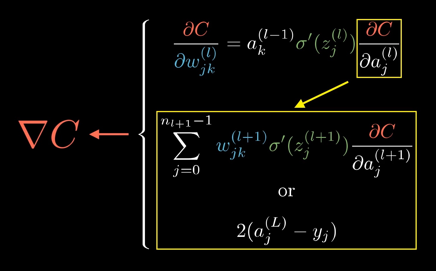
A large portion of the math for calculating the gradient using backpropagation is captured in this image.
These chain rule expressions are the derivatives that make up the gradient vector, which lets us minimize the cost of the network by repeatedly stepping downhill. If you sit back and think about it, that's a lot of layers of complexity to wrap your mind around, and it takes time for your mind to digest it all.
These formulas are usually encapsulated more neatly into a few nice vector expressions, so all the messy indices aren't out in the open.
Given that you'd typically have the actual implementation handled by a library for you, the most important and generalizable understanding here is how you can reason about the sensitivity of one variable to another by breaking down the chain of dependencies.
Stepping back, if you take away just one idea from this series, I want you to reflect on how even relatively simple pieces of math, like matrix multiplication and derivatives, can enable you to build genuinely incredible technology when put into the right context.
Think about how matrix multiplication elegantly captures the propagation of information from one layer of neurons to the next. Think about how we can take the somewhat fuzzy idea of intelligence, or at least the narrow sliver of intelligence required to classify images correctly, and turn it into a piece of calculus by finding the minimum of a carefully defined cost function. Think about how derivatives and gradients give us a concrete way to find such a minimum (well, a local minimum anyway). Or think about the chain rule, which in most calculus classes comes across as "just one of those tools" that you need for more homework problems, and how in this context it let us cleanly decompose an insanely complicated network of influences to understand how sensitive that cost function is to each and every weight and bias.
Additional Resources
This marks the end of our series together, but there is always more to learn! If you want to dive even deeper into the calculus of backpropagation, I recommend these resources:
- http://neuralnetworksanddeeplearning.com/chap2.html
- https://github.com/mnielsen/neural-networks-and-deep-learning
- http://colah.github.io/posts/2015-08-Backprop/
And if you're interested in diving deeper into this topic as a whole, I highly recommend the book by Michael Nielsen on deep learning and neural networks. In it, you can find the code and data to download to play with for this exact example, and he walks you through step-by-step what that code is doing.
What's awesome is that the book is free and publicly available, so if you get something out of it, consider joining me in making a donation to Nielsen's efforts.
Also check out Chris Olah's blog. His post on Neural networks and topology is particularly beautiful, but honestly all of the stuff there is great. And if you like that, you'll love the publications at Distill.
For more videos, Welch Labs also has some great series on machine learning:
"But I've already voraciously consumed Nielsen's, Olah's and Welch's works," I hear you say. Well well, look at you then. That being the case, I might recommend that you continue on with the book "Deep Learning" by Goodfellow, Bengio, and Courville.
Thanks
Special thanks to those below for supporting this lesson.