Eigenvectors and eigenvalues
Eigenvalues and eigenvectors are one of the most important ideas in linear algebra, but what on earth are they?
Last time, I asked: 'What does mathematics mean to you?', and some people answered: 'The manipulation of numbers, the manipulation of structures.' And if I had asked what music means to you, would you have answered: 'The manipulation of notes?'
- Serge Lang
Eigenvectors and eigenvalues are some of those topics that a lot of students find particularly unintuitive. Questions like "why are we doing this?" and "what does this actually mean?" are too often left floating away unanswered in a sea of computations. And as I've put out chapters in this series, many of you have commented about looking forward to visualizing this topic in particular.
I suspect that the reason for this is not so much that eigen-things are particularly complicated or poorly explained. In fact, it's comparatively straightforward, and I think most books do a fine job explaining it. The issue is that it only really makes sense if you have a solid visual understanding of many of the topics that precede it. Most important here is that you know how to think about matrices as linear transformations. But you also need to be comfortable with , , and . Confusion about eigen-stuffs usually has more to do with a shaky foundation in one of these topics than it does with the eigenvectors and eigenvalues themselves.
An example
To start, consider some linear transformation in two dimensions, like the one shown here.

It moves the basis vector \hat{\imath} to the coordinates \left[\begin{array}{c}3 \\ 0\end{array}\right], and \hat{\jmath} to \left[\begin{array}{c}1 \\ 2\end{array}\right], so it's represented with a the matrix \left[\begin{array}{c}3 & 1 \\ 0 & 2\end{array}\right]. Now, focus on what it does to any individual vector, and think about the span of that vector, which is the line passing through the origin and its tip.

Most vectors will get knocked off that line during the transformation. It would seem pretty coincidental if the place where a vector lands happens to be somewhere on that line. But some special vectors do remain on their own span, meaning the effect the matrix has on such a vector is to just stretch or squish it, like a scalar.

For this specific example, the basis vector \hat{\imath} is one such vector with this special property. The span of \hat{\imath} is the x-axis, and from the first column of the matrix we can see that \hat{\imath} moves over to 3 times itself, still on that x-axis. What's more, because of the way linear transformations work, any other vector on the x-axis is also just stretched by a factor of 3, and hence remains on its own span.

A slightly sneakier vector that remains on its own span during this transformation is \left[\begin{array}{c}1 \\ -1\end{array}\right]. It ends up getting stretched out by a factor of 2. And again, linearity will imply that any other vector on the diagonal line spanned by this one will just get stretched out by a factor of 2.

For this transformation, those are all the vectors with this special property of staying on their span: Those on the x-axis that get stretched by a factor of 3, and those on this diagonal line that are stretched by a factor of 2. Any other vector will get rotated somewhat during the transformation, knocked off of the line it spans.

These special vectors are called the "eigenvectors" of the transformation, and each eigenvector has associated with it what's called an "eigenvalue", which is the factor by which it's stretched or squished during the transformation. In this example, vectors on the x-axis are eigenvectors with eigenvalue 3, while those on the diagonal line are eigenvectors with eigenvalue 2.

Of course, there's nothing special about stretching vs. squishing, or the fact that these eigenvalues happen to be positive. In another example you could have an eigenvector with eigenvalue -\frac{1}{2}, meaning that vector gets flipped and squished by a factor of \frac{1}{2}, but the important part is that it stays on the line that it spans out, without being rotated off of it.

Eigenvector with eigenvalue -\frac{1}
{2}.
3d rotational axis
For a glimpse of why this might be a useful thing to think about, consider some three-dimensional rotation. If you can find an eigenvector for this rotation, a vector which remains on its own span, what you have found is the axis of rotation.

It's much easier to think about a 3d rotation in terms of an axis of rotation, and an angle by which it is rotating, rather than thinking about the full 3x3 matrix associated with such a transformation.
3d rotational axis


In this case, the corresponding eigenvalue would have to be 1, since 3d rotations don't stretch or squish anything.
This is a pattern that shows up a lot in linear algebra: With any linear transformation described by a matrix, you could understand what it's doing by reading off the columns of this matrix as the landing spots for the basis vectors. But often a better way to get at the heart of what that transformation actually does, less dependent on your particular coordinate system, is to find the eigenvectors and eigenvalues.
Notes on computation
We won't cover the full details on methods for computing eigenvectors and eigenvalues here, but we'll try to give an overview of the computational ideas that are most important for conceptual understanding.
Symbolically, here's what the idea of eigenvectors and eigenvalues looks like. A is the matrix representing some transformation, with \vec{\mathbf{v}} as an eigenvector, and \lambda (lambda) is a number, namely the corresponding eigenvalue.

What this expression is saying is that the matrix-vector product A times \vec{\mathbf{v}} gives the same result as scaling the eigenvector \vec{\mathbf{v}} by the eigenvalue lambda.

Finding the eigenvectors and eigenvalues of a matrix A comes down to finding values of \mathbf{v} and \lambda that make this expression true. It's a little awkward to work with at first, because the left-hand-side represents matrix vector multiplication, while the right-hand-side is scalar-vector multiplication. Let's start by rewriting that right-hand-side as some kind of matrix vector multiplication, using a matrix which has the effect of scaling vectors by a factor of lambda.

The columns of such matrix will represent what happens to each basis vector, and each basis vector is simply multiplied by lambda, so this matrix will have the number lambda down the diagonal with zeros everywhere else. The common way to write this matrix is as lambda times I, where I is the identity matrix with 1s down the diagonal.

With both sides looking like matrix-vector multiplication, we can subtract off the right-hand side and factor out the \vec{\mathbf{v}}. So we have a new matrix, \left(A - \lambda I\right), and we're looking for a vector \vec{\mathbf{v}} such that this new matrix times \vec{\mathbf{v}} gives the zero vector.

Now, this will always be true when \vec{\mathbf{v}} is the zero vector, but that's boring, we want a non-zero eigenvector.
Zero Determinant
As viewers of and will know, the only way it's possible for the product of a matrix with a nonzero vector to become zero is if the transformation associated with that matrix squishes space into a lower dimension. And that squishification corresponds to a zero determinant of the matrix.

To be concrete, let's say your matrix is \left[\begin{array}{c} 2 & 2 \\ 1 & 3 \end{array}\right], and imagine subtracting off the variable amount lambda from each diagonal entry.

Imagine tweaking lambda, turning a knob to change its value. As that value of lambda changes, the matrix changes, and so the determinant of that matrix changes.

The goal is to find a value of lambda that will make the determinant zero, meaning the tweaked transformation squishes space. In this case, the sweet spot comes when \lambda = 1.

Remember that the lambda is tied to the matrix, so if we use another matrix, the lambda might not be 1. To unravel what that means, when \lambda=1, the matrix A - \lambda \cdot I squishes space onto a line. That means there's a nonzero vector \mathbf{v} such that (A-\lambda\cdot I)\cdot \mathbf{v}=0.
The reason we care about that is because it means A \cdot \mathbf{v} = \lambda \cdot \mathbf{v}, which you can read as saying the vector \mathbf{v} is an eigenvector of A, staying on its own span during the transformation A. In this example, the corresponding eigenvalue is 1, so it actually just stays fixed in place.
\begin{aligned}
A \vec{\mathbf{v}} & =\lambda \vec{\mathbf{v}} \\ \rule{0pt}{2em}
A \vec{\mathbf{v}}-\lambda I \vec{\mathbf{v}} & =0 \\ \rule{0pt}{2em}
(A-\lambda I) \vec{\mathbf{v}} & =0 \\ \rule{0pt}{2em}
\operatorname{det}(A-\lambda I) & =0
\end{aligned}
Pause and ponder to make sure that line of reasoning feels good.
Characteristic polynomial
This expression, where we take a given matrix minus lambda times the identity and set its determinant equal to zero, thinking of lambda as a variable, is fundamental to eigenvalues. This is the kind of thing we mentioned in the introduction. If you didn't have a solid grasp of the determinant, and why it relates to linear systems having non-zero solutions, an expression like this would feel completely out of the blue.
Let's revisit the example from the start, with the matrix \left[\begin{array}{c} 3 & 1\\ 0 & 2 \end{array}\right].

To find if a value \lambda is an eigenvalue, subtract it from the diagonals of this matrix, and compute the determinant.
\operatorname{det}\left(\left[\begin{array}{cc}3-\lambda & \mathbb{1} \\ 0 & 2-\lambda\end{array}\right]\right)Doing this, we get a certain quadratic polynomial in terms of lambda.
\operatorname{det}\left(\left[\begin{array}{cc}3-\lambda & \mathbb{1} \\ 0 & 2-\lambda\end{array}\right]\right) = (3 - \lambda)(2- \lambda)Since lambda can only be an eigenvalue if this determinant is zero, you can conclude that the only eigenvalues are \lambda = 2 and \lambda = 3. To see what eigenvectors have one of these eigenvalues, say \lambda=2, plug in that value of lambda to the matrix, and solve for which vectors this diagonally-altered matrix sends to zero.
\left[\begin{array}{cc}
3-2 & 1 \\
0 & 2-2
\end{array}\right]\left[\begin{array}{l}
x \\
y
\end{array}\right]=\left[\begin{array}{l}
0 \\
0
\end{array}\right]
If you computed this, you'd see that the solutions are all of the vectors on the diagonal line spanned by \left[\begin{array}{c} -1 \\ 1 \end{array}\right]. This corresponds to the fact that the unaltered matrix \left[\begin{array}{c} 3 & 1 \\ 0 & 2 \end{array}\right] stretches all those vectors by a factor of 2.

Rotation
Now, a 2d transformation doesn't have to have eigenvectors. For example, consider a rotation by 90 degrees. This doesn't have any eigenvectors, since each vector is rotated off of its own span.

If you actually try computing the eigenvalues for a 90 degree rotation, notice what happens. Its matrix is \left[\begin{array}{c} 0 & -1 \\ 1 & 0 \end{array}\right]. Subtract \lambda from the diagonal elements, and look for when the determinant is 0.
\begin{aligned}
\operatorname{det}\left(\left[\begin{array}{cc}-\lambda & -1 \\ 1 & -\lambda\end{array}\right]\right) & =(-\lambda)(-\lambda)-(-1)(1) \\ \rule{0pt}{2em}
& =\lambda^2+1=0
\end{aligned}
In this case, you get the polynomial \lambda^2 + 1. The only roots of this polynomial are the imaginary numbers i and -i. The fact that there are no real number solutions indicates that there are no eigenvectors.
Shear
Another interesting example is a shear. This fixes \hat{\imath} in place, and moves \hat{\jmath} one over, so its matrix is \left[\begin{array}{c} 1 & 1 \\ 0 & 1\end{array}\right].

All the vectors on the x-axis are eigenvectors with eigenvalue 1, since they remain fixed in place. In fact these are the only eigenvectors. When you subtract \lambda from the diagonals and compute the determinant, you get (1-\lambda)^2, and the only root of that expression is \lambda = 1.
\operatorname{det}\left(\left[\begin{array}{cc}
1-\lambda & 1 \\
0 & 1-\lambda
\end{array}\right]\right)=\underbrace{(1-\lambda)(1-\lambda)=0}_{\lambda=1}
This lines up with what we see geometrically that all the eigenvectors have eigenvalue 1.

Scaling
It's also possible to have just one eigenvalue with more than just a line full of eigenvectors. A simple example is the matrix which scales everything by 2. The only eigenvalue is 2, but every vector in the plane gets to be an eigenvector with that eigenvalue.

Scale everything by 2.
Now is another good time to pause and ponder some of this.
Questions
Working in an eigenbasis
Let's finish off here with the idea of an eigenbasis, which relies heavily on ideas from the last chapter.
Take a look at what happens if our basis vectors happen to be eigenvectors. For example, maybe \hat{\imath} is scaled by -1, and \hat{\jmath} is scaled by 2. Writing their new coordinates as columns of a matrix, notice that those scalar multiples -1 and 2, which are the eigenvalues of \hat{\imath} and \hat{\jmath}, are on the diagonal, and all other entries are 0.

Any time a matrix has zeros everywhere other than the diagonal, it's called a "diagonal matrix", and the way to interpret it is that all the basis vectors are eigenvectors, and the diagonal entries of the matrix give you their corresponding eigenvalues.
\left[\begin{array}{cccc}
-5 & 0 & 0 & 0 \\
0 & -2 & 0 & 0 \\
0 & 0 & -4 & 0 \\
0 & 0 & 0 & 4
\end{array}\right]
There are a number of things that make diagonal matrices nicer to work with. One big one is that it's easier to compute what will happen if you multiply this matrix by itself a whole bunch of times.
\begin{aligned}
\left[\begin{array}{ll}
3 & 0 \\
0 & 2
\end{array}\right]
\left[\begin{array}{l}
x \\
y
\end{array}\right]
& =
\left[\begin{array}{c}
3 x \\
2 y
\end{array}\right] \\ \rule{0pt}{2.5em}

\left[\begin{array}{ll}
3 & 0 \\
0 & 2
\end{array}\right]
\left[\begin{array}{c}
3 x \\
2 y
\end{array}\right]
& =
\left[\begin{array}{c}
3^2 x \\
2^2 y
\end{array}\right] \\ \rule{0pt}{2.5em}

\left[\begin{array}{ll}
3 & 0 \\
0 & 2
\end{array}\right]
\left[\begin{array}{c}
3^2 x \\
2^2 y
\end{array}\right]
& =
\left[\begin{array}{c}
3^3 x \\
2^3 y
\end{array}\right] \\ \rule{0pt}{2.5em}

& \ldots
\end{aligned}
Since all one of these matrices does is scale each basis vector by some eigenvalue, applying that matrix, say, 100 times will just correspond to scaling each basis vector by the 100th power of the corresponding eigenvalue.
\underbrace{\left[\begin{array}{ll}
3 & 0 \\
0 & 2
\end{array}\right] \cdots \left[\begin{array}{ll}
3 & 0 \\
0 & 2
\end{array}\right]\left[\begin{array}{ll}
3 & 0 \\
0 & 2
\end{array}\right]\left[\begin{array}{ll}
3 & 0 \\
0 & 2
\end{array}\right]}_{100 \text { times }}\left[\begin{array}{l}
x \\
y
\end{array}\right]
=
\left[\begin{array}{cc}
3^{100} & 0 \\
0 & 2^{100}
\end{array}\right]\left[\begin{array}{l}
x \\
y
\end{array}\right]
By contrast, consider how hard computing the 100th power of a non-diagonal matrix would be. Really, think about it for a moment, compared to simply exponentiating the entries it's a nightmare!
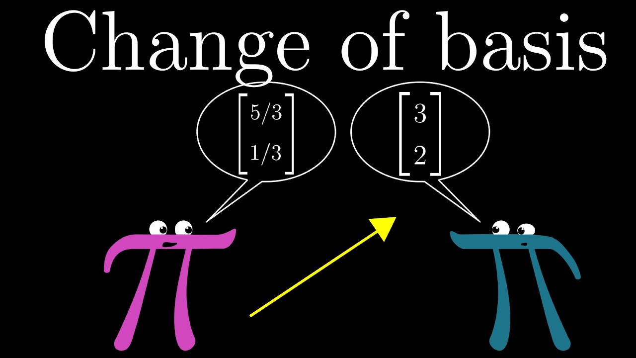
Change of basis
Of course, you will rarely be so lucky as to have your basis vectors also be eigenvectors. But if your transformation has lots of eigenvectors, enough that you can choose a set that spans the full space, then you can change your coordinate system so that these eigenvectors are your basis vectors.

We talked all about change of basis in the , but let's go through a super quick reminder here of how to express a transformation in a different coordinate system.
Take the coordinates of the vectors you want to use as a basis, which in our cases means two eigenvectors, then make those coordinates the columns of a matrix, known as the change of basis matrix. When you sandwich the original transformation, putting the change of basis matrix on its right and the inverse change of basis matrix on its left, the result will be a matrix representing this same transformation, but from the perspective of the new basis vector's coordinate system.

The whole point of doing this with eigenvectors is that this new matrix is guaranteed to be diagonal, with the corresponding eigenvalues down the diagonal, since this represents working in a coordinate system where basis vectors just get scaled during the transformation.

A set of basis vectors which are all also eigenvectors is called an "eigenbasis". For example, if you needed to compute the 100th power of this matrix, it would be much easier to change to an eigenbasis, compute the 100th power in that system, then convert back to the standard system. You can't do this with all transformations. A shear, for example, doesn't have enough eigenvectors to span all of space. But if you can find an eigenbasis, it can make matrix operations really lovely.
For anyone willing to work through a neat puzzle to see what this looks like in action, and how it can be used to produce surprising results, we'll put the puzzle prompt below. It's a bit of work, but we think you'll enjoy it.
Take the following matrix:
A=\left[\begin{array}{ll}
0 & 1 \\
1 & 1
\end{array}\right]
Start computing its first few powers by hand: A^2, A^3, etc. What pattern do you see? Can you explain why this pattern shows up? This might make you curious to know if there's an efficient way to compute arbitrary powers of this matrix, A^n for any number n.
Given that two eigenvectors of this matrix are
\overrightarrow{\mathbf{v}}_1=\left[\begin{array}{c}
\frac{1}{2}(-1 + \sqrt{5}) \\
1
\end{array}\right] \quad \overrightarrow{\mathbf{v}}_2=\left[\begin{array}{c}
\frac{1}{2}(-1 - \sqrt{5}) \\
1
\end{array}\right],
see if you can figure out a way to compute A^n by first changing to an eigenbasis, compute the new representation of A^n in that basis, then converting back to our standard basis. What does this formula tell you?
Eigenvector puzzle solution
In the puzzle we were given the following matrix,
\begin{align*}
	A = \left[
	        	\begin{array}{cc}
			0 & 1 \\
			1 & 1
        		\end{array}
	\right],
\end{align*}
and we were asked to compute several powers of this matrix. Taking the time to work out the first few, here's what we get.
\begin{align*}
	A^2 &= \left[
	        	\begin{array}{cc}
			0 & 1 \\
			1 & 1
        		\end{array}
	\right]
	 \left[
	        	\begin{array}{cc}
			0 & 1 \\
			1 & 1
        		\end{array}
	\right] =
	 \left[
	        	\begin{array}{cc}
			1 & 1 \\
			1 & 2
        		\end{array}
	\right] \\\\
	A^3 = A A^2 &= \left[
	        	\begin{array}{cc}
			0 & 1 \\
			1 & 1
        		\end{array}
	\right]
	 \left[
	        	\begin{array}{cc}
			1 & 1 \\
			1 & 2
        		\end{array}
	\right] =
	 \left[
	        	\begin{array}{cc}
			1 & 2 \\
			2 & 3
        		\end{array}
	\right] \\\\
	A^4 = A A^3 &= \left[
	        	\begin{array}{cc}
			0 & 1 \\
			1 & 1
        		\end{array}
	\right]
	 \left[
	        	\begin{array}{cc}
			1 & 2 \\
			2 & 3
        		\end{array}
	\right] =
	 \left[
	        	\begin{array}{cc}
			2 & 3 \\
			3 & 5
        		\end{array}
	\right] \\\\
	A^5 = A A^4 &= \left[
	        	\begin{array}{cc}
			0 & 1 \\
			1 & 1
        		\end{array}
	\right]
	 \left[
	        	\begin{array}{cc}
			2 & 3 \\
			3 & 5
        		\end{array}
	\right] =
	 \left[
	        	\begin{array}{cc}
			3 & 5 \\
			5 & 8
        		\end{array}
	\right] \\\\
	A^6 = A A^5 &= \left[
	        	\begin{array}{cc}
			0 & 1 \\
			1 & 1
        		\end{array}
	\right]
	 \left[
	        	\begin{array}{cc}
			3 & 5 \\
			5 & 8
        		\end{array}
	\right] =
	 \left[
	        	\begin{array}{cc}
			5 & 8 \\
			8 & 13
        		\end{array}
	\right] \\\\
\end{align*}
Two things stand out as we do this. First, this process is tedious! Finding matrix powers is no fun, and the prospect of finding something like A^{100} feels truly horrifying. And even if you have a computer to evaluate this for you, finding matrix powers simply by repeating matrix multiplication stands to be very computationally inefficient, especially for large matrices. Switching to an eigenbasis, as you are about to see, can greatly speed up the process, both for doodling humans and number-crunching machines.
The second thing that stands out is that the terms in side our matrix appear to be following the Fibonacci sequence! 1, 1, 2, 3, 5, 8, 13, \dots There's actually a good reason for this. Notice how this matrix acts on an arbitrary vector:
\begin{align*}
	 \left[
	        	\begin{array}{cc}
			0 & 1 \\
			1 & 1
        		\end{array}
	\right]
	 \left[
	        	\begin{array}{c}
			a \\
			b
        		\end{array}
	\right] =
	 \left[
	        	\begin{array}{c}
			b \\
			a+b
        		\end{array}
	\right] \\\\
\end{align*}
So the second component of the input, b, vector gets shifted to be the first component of the output, and the second component of the output becomes the sum of a and b. For example, think of applying that process repeatedly to a given vector:
\begin{align*}
	 \left[
	        	\begin{array}{c}
			a \\
			b
        		\end{array}
	\right] &\rightarrow
	 \left[
	        	\begin{array}{c}
			b \\
			a+b
        		\end{array}
	\right] \\ \quad \\
	 \left[
	        	\begin{array}{c}
			1 \\
			1
        		\end{array}
	\right] \rightarrow
	 \left[
	        	\begin{array}{c}
			1 \\
			2
        		\end{array}
	\right] \rightarrow
	 \left[
	        	\begin{array}{c}
			2 \\
			3
        		\end{array}
	\right] &\rightarrow
	 \left[
	        	\begin{array}{c}
			3 \\
			5
        		\end{array}
	\right] \rightarrow
	 \left[
	        	\begin{array}{c}
			5 \\
			8
        		\end{array}
	\right] \rightarrow
	 \left[
	        	\begin{array}{c}
			8 \\
			13
        		\end{array}
	\right] \rightarrow \cdots
\end{align*}
This iterative process perfectly capture the one defining the Fibonacci sequence: Each term is the sum of the previous two terms.
Since multiplying the matrix A^n by a vector corresponds to going through this process n times, figuring out how to represent A^n can lead us to an explicit formula for the nth Finbonacci term. I don't know about you, but I find that awesome! Well, maybe it's not obvious that a clean formula for A^n is achievable, but this is where eigenvectors come in.
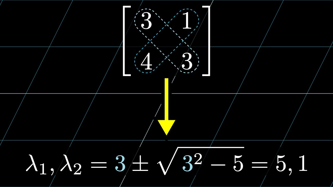
We can find the eigenvalues of this matrix by subtracting a variable \lambda off the diagonal, and computing when its determinant is 0:
\begin{align*}
	\det(A - \lambda I) =
	\det\left(\left[
		\begin{array}{cc}
			0 - \lambda & 1 \\
			1 & 1 - \lambda
		\end{array}
	\right]\right) =
	\lambda^2 - \lambda  - 1 = 0
\end{align*}
This quadratic has two solutions:
\begin{align*}
	\lambda_1 &= \frac{1 + \sqrt{5}}{2} \\
	\lambda_2 &= \frac{1 - \sqrt{5}}{2} \\
\end{align*}
Some of you may recognize the first of these as the golden ratio \varphi = 1.618\dots, and the second as -\frac{1}{\varphi} = -0.618\dots.
To find the eigenvectors, you find a non-zero solution to the equation
\begin{align*}
	\left[
		\begin{array}{cc}
			0 - \lambda & 1 \\
			1 & 1 - \lambda
		\end{array}
	\right]
	\left[
		\begin{array}{c}
			x \\
			y
		\end{array}
	\right] =
	\left[
		\begin{array}{c}
			0 \\
			0
		\end{array}
	\right]
\end{align*}
Doing so, you'll find that the eigenvectors corresponding to \lambda_1 and \lambda_2 are
\begin{align*}
	\textbf{v}_1 &= \left[
		\begin{array}{c}
			\frac{1}{2}(-1 + \sqrt{5}) \\
			1
		\end{array}
	\right] \\ \quad \\
	\textbf{v}_2 &= \left[
		\begin{array}{c}
			\frac{1}{2}(-1 - \sqrt{5}) \\
			1
		\end{array}
	\right]
\end{align*}
Why are we doing this? Well, think about what it means for \textbf{v}_1 to be an eigenvector of A. It means multiplying A by \textbf{v}_1 just has the effect of scaling it by a constant, namely the eigenvalue \lambda_1. So repeatedly multiplying A by this vector, say 100 times, just has the effect of scaling this vector by \lambda_1^{100}. So, if we switch to a coordinate system where the two eigenvalues are our basis, the action A^n will have a very simple form, since its effect on the basis vectors would simply be multiplying by \lambda_1^n and \lambda_2^n.
So...how do you switch to a different basis? If you'll recall from the last lesson, a matrix whose columns are the vectors \textbf{v}_1 and \textbf{v}_2 can be thought of as translating a coordinates describing a certain vector in the language of that basis system into a description of that same vector in our basis. That is, define the matrix
\begin{align*}
	S = \left[
		\begin{array}{cc}
			\frac{1}{2}(-1 + \sqrt{5}) & \frac{1}{2}(-1 - \sqrt{5}) \\
			1 & 1
		\end{array}
	\right].
\end{align*}
Then S is the change of basis matrix which has the effect of taking in a vector written in the coordinates of the eigenbasis, and spitting out the coordinates for that same vector in our standard basis. So to take the action of the matrix A, and write it in the language of the eigenbasis, we'd write an expression like this:
\begin{align*}
	D = S^{-1} A S
\end{align*}
You might read the right side here as saying first translate from the language of the eigenbasis to our basis, then apply A, then translate back. The resulting matrix D will represent the same transformation as A, just in the language of the eigenbasis. The whole point of doing this is to make it so that the action of A just looks like stretching two basis vectors. Let's see how that plays out!
The inverse of S is
\begin{align*}
	S^{-1} = \left[
		\begin{array}{cc}
			\frac{1}{2}(-1 + \sqrt{5}) & \frac{1}{2}(-1 - \sqrt{5}) \\
			1 & 1
		\end{array}
	\right]^{-1}
	=
	\frac{1}{\det(S)} \left[
		\begin{array}{cc}
			1 & -\frac{1}{2}(-1 - \sqrt{5}) \\
			-1 & \frac{1}{2}(-1 + \sqrt{5})
		\end{array}
	\right]
	=
	\frac{1}{\sqrt{5}} \left[
		\begin{array}{cc}
			1 & -\frac{1}{2}(-1 - \sqrt{5}) \\
			-1 & \frac{1}{2}(-1 + \sqrt{5})
		\end{array}
	\right]
\end{align*}
Crunching through it all, we then get
\begin{align*}
	D = S^{-1}AS
	&=
	\frac{1}{\sqrt{5}} \left[
		\begin{array}{cc}
			1 & -\frac{1}{2}(-1 - \sqrt{5}) \\
			-1 & \frac{1}{2}(-1 + \sqrt{5})
		\end{array}
	\right]
	\left[
		\begin{array}{cc}
			0 & 1 \\
			1 & 1
		\end{array}
	\right]
	 \left[
		\begin{array}{cc}
			\frac{1}{2}(-1 + \sqrt{5}) & \frac{1}{2}(-1 - \sqrt{5}) \\
			1 & 1
		\end{array}
	\right] \\\\
	&=
	\frac{1}{\sqrt{5}} \left[
		\begin{array}{cc}
			1 & -\frac{1}{2}(-1 - \sqrt{5}) \\
			-1 & \frac{1}{2}(-1 + \sqrt{5})
		\end{array}
	\right]
	 \left[
		\begin{array}{cc}
			1 & 1 \\
			\frac{1}{2}(1 + \sqrt{5}) & \frac{1}{2}(1 - \sqrt{5})
		\end{array}
	\right] \\\\
	&=
	 \left[
		\begin{array}{cc}
			\frac{1}{2}(1 + \sqrt{5}) & 0 \\
			0 & \frac{1}{2}(1 - \sqrt{5})
		\end{array}
	\right] \\\\
	&=
	 \left[
		\begin{array}{cc}
			\lambda_1 & 0 \\
			0 & \lambda_2
		\end{array}
	\right] \\\\
\end{align*}
We actually could have concluded this ahead of time, since the action of A on the first eigenvector is to scale it by \lambda_1 = \frac{1}{2}(1 + \sqrt{5}), and its action on the second basis vector is to scale it by \lambda_1 = \frac{1}{2}(1 - \sqrt{5}). Nevertheless, it's nice to get a little computational confirmation now and then.
Okay, final stretch! This means in the eigenbases, the action of our transformation n times is simply
\begin{align*}
	D^n =
	 \left[
		\begin{array}{cc}
			\lambda_1 & 0 \\
			0 & \lambda_2
		\end{array}
	\right]^n =
	 \left[
		\begin{array}{cc}
			\lambda_1^n & 0 \\
			0 & \lambda_2^n
		\end{array}
	\right]
\end{align*}
Compare that to how it felt to compute the first few powers of A^n, much easier! Of course, this is all in coordinate system of the eigenbasis, so to translate back to our coordinate system, we have
\begin{align*}
	A^n =
	S(D^n)S^{-1} &=
	 \left[
		\begin{array}{cc}
			\frac{1}{2}(-1 + \sqrt{5}) & \frac{1}{2}(-1 - \sqrt{5}) \\
			1 & 1
		\end{array}
	\right]
	 \left[
		\begin{array}{cc}
			\lambda_1^n & 0 \\
			0 & \lambda_2^n
		\end{array}
	\right]
	\frac{1}{\sqrt{5}} \left[
		\begin{array}{cc}
			1 & -\frac{1}{2}(-1 - \sqrt{5}) \\
			-1 & \frac{1}{2}(-1 + \sqrt{5})
		\end{array}
	\right] \\\\
\end{align*}
This can be a written a little more nicely if we notice the occurrence of \lambda_1 = \frac{1}{2}(1 + \sqrt{5}) and \lambda_2 = \frac{1}{2}(1 - \sqrt{5}) in the change of basis matrices, and pull the \frac{1}{\sqrt{5}} term to the front. Also, in doing the calculuation, I'll take advantage of the convenient fact that \lambda_1\lambda_2 = -1
\begin{align*}
	A^n =
	S(D^n)S^{-1} &=
	\frac{1}{\sqrt{5}}
	 \left[
		\begin{array}{cc}
			-\lambda_2 & -\lambda_1 \\
			1 & 1
		\end{array}
	\right]
	 \left[
		\begin{array}{cc}
			\lambda_1^n & 0 \\
			0 & \lambda_2^n
		\end{array}
	\right]
	\left[
		\begin{array}{cc}
			1 & \lambda_1 \\
			-1 & -\lambda_2
		\end{array}
	\right] \\\\
	&=
	\frac{1}{\sqrt{5}}
	 \left[
		\begin{array}{cc}
			-\lambda_2 & -\lambda_1 \\
			1 & 1
		\end{array}
	\right]
	 \left[
		\begin{array}{cc}
			\lambda_1^n & \lambda_1^{n+1} \\
			-\lambda_2^n & -\lambda_2^{n+1}
		\end{array}
	\right] \\\\
	&=
	\frac{1}{\sqrt{5}}
	 \left[
		\begin{array}{cc}
			-\lambda_2 \lambda_1^{n} + \lambda_1 \lambda_2^n & -\lambda_2 \lambda_1^{n+1} + \lambda_1 \lambda_2^{n+1} \\
			\lambda_1^n - \lambda_2^n & \lambda_1^{n+1} - \lambda_2^{n+1}
		\end{array}
	\right] \\\\
	&=
	\frac{1}{\sqrt{5}}
	 \left[
		\begin{array}{cc}
			\lambda_1^{n-1} - \lambda_2^{n-1} & \lambda_1^{n} - \lambda_2^{n} \\
			\lambda_1^n - \lambda_2^n & \lambda_1^{n+1} - \lambda_2^{n+1}
		\end{array}
	\right] \\\\
\end{align*}
If you compare this to the first few computations we did for A^n at the start, this gives us a very striking formula. The nth Fibonacci number has the formula
\begin{align*}
	F_n = \frac{\lambda_1^n - \lambda_2^n}{\sqrt{5}}
	= \frac{\left(\frac{1 + \sqrt{5}}{2}\right)^n - \left(\frac{1 - \sqrt{5}}{2}\right)^n}{\sqrt{5}}
\end{align*}
It's not even obvious that this expression should give a rational expression, much less the Fibonacci numbers!
The next chapter is about a quick trick for computing eigenvalues before the final chapter of the series on abstract vector spaces.