Gradient descent, how neural networks learn
An overview of gradient descent in the context of neural networks. This is a method used widely throughout machine learning for optimizing how a computer performs on certain tasks.
In the last lesson we explored the structure of a neural network. Now, let's talk about how the network learns by seeing many labeled training data. The core idea is a method known as gradient descent, which underlies not only how neural networks learn, but a lot of other machine learning as well.
Recap From Last Time
As a reminder, our goal is to recognize handwritten digits. It's a classic example—the "hello world" of neural networks.

Our goal is to recognize these handwritten digits.
These digits are rendered onto a 28x28 pixel grid, where each pixel has some grayscale value between 0.0 and 1.0. Those 784 values determine the activations of the neurons in the input layer of the network.
Each pixel value in the image becomes the activation of a particular neuron in the first layer of the network.
The activation for each neuron in the following layers is based on a weighted sum of all activations from the previous layer, plus some number called the "bias." We then wrap a nonlinear function around this sum, such as a sigmoid or a ReLU.
a_{0}^{(1)} =
\textcolor{#d69d00}{
\sigma\left(
\textcolor{black}{

\textcolor{green}{w_{0,0}} a_{0}^{(0)} +
\textcolor{green}{w_{0,1}} a_{1}^{(0)} +
\cdots +
\textcolor{green}{w_{0,n}} a_{n}^{(0)}
\textcolor{blue}{+ b_{0}}

}
\right)
}
In this way, values propagate from one layer to the next, entirely determined by the weights and biases. The brightest of the ten neurons in the output layer is the network's choice for which digit the image represents.

The input layer of neurons has activations based on the pixel values of an image. The rest of the layers have activations depending on each previous layer.
In total, given the somewhat arbitrary choice of 2 hidden layers with 16 neurons each, this network has 13,002 weights and biases that we can adjust, and it's these values that determine what exactly the network does.
Remember, the motivation we had in mind for this layered structure was that maybe the second layer could pick up on edges, the third on patterns like loops and lines, and the last one pieces together those patterns to recognize digits:

We hope that the layered structure might allow the problem to be broken into smaller steps, from pixels to edges to loops and lines, and finally to digits.
How the Network Learns
What makes machine learning different from other computer science is that you don't explicitly write instructions for doing a particular task. In this case, you never actually write an algorithm for recognizing digits. Instead, you write an algorithm that can take in a bunch of example images of handwritten digits along with labels for what they are and adjust those 13,002 weights and biases of the network to make it perform better on those examples.
The labeled images we feed in are collectively known as the "training data".

The network learns by looking at examples of correctly identified digits.
Hopefully, the layered structure will mean that what it learns generalizes to images beyond the training data. To test this, after training the network, we can show it more labeled data that it's never seen before and see how accurately it classifies them.

We use some of the data for training the network and some other data it's never seen before for testing it after it's trained.
This process requires a lot of data. Fortunately, the good people behind the MNIST database have put together a collection of tens of thousands of handwritten digit images, each labeled with the number they are supposed to be, that we can use for free.
I should point out that although it can be provocative to describe a machine as "learning", once you see how it works, it feels a lot less like some crazy sci-fi premise and a lot more like a calculus exercise. It really just comes down to finding the minimum of a specific function.

The process of learning is essentially just finding lower and lower points on a specific function.
The Cost Function
Remember, our network's behavior is determined by all of its weights and biases. The weights represent the strength of connections between each neuron in one layer and each neuron in the next. And each bias is an indication of whether its neuron tends to be active or inactive.

The behavior of the network depends on its weights and biases.
To start things off, initialize all the weights and biases to be random numbers. This network will perform horribly on the given training example since it's just doing something random.
For example, if you feed in this image of a 3, the output layer just looks like a mess:

Initialized with totally random weights and biases, the network is terrible at identifying digits.
So how do you programmatically identify that the computer is doing a lousy job and then help it improve?
What you do is define a cost function, which is a way of telling the computer, "No, bad computer, that output layer should have activations which are 0 for most neurons, but with a 1 for the third neuron. What you gave me is utter trash!"

We measure how badly the network is doing by comparing its results to the correct answer.
To say that a little more mathematically, add up the squares of the differences between each of these trash output activations and the values you want them to have. We'll call this the "cost" of a single training example.

The cost is small when the network confidently classifies this image correctly but large when it doesn't know what it's doing.

The Cost Over Many Examples
But we aren't just interested in how the network performs on a single image. To really measure its performance, we need to consider the average cost over all the tens of thousands of training examples. This average is our measure of how lousy the network is and how bad the computer should feel.
This is, to put it lightly, a complicated function. Remember how the network itself is a function? It has 784 inputs (the pixel values), 10 outputs, and 13,002 parameters.

The neural network is a function that takes in images and spits out digit predictions based on the weights and biases.
The cost function is a layer of complexity on top of that. The inputs of the cost function are those 13,002 weights and biases, and it spits out a single number describing how bad those weights and biases are. It's defined in terms of the network's behavior on all the tens of thousands of pieces of labeled training data. In other words, this training data is a massive set of parameters to the cost function.

The cost function takes in the weights and biases of a network and uses the training images to compute a "cost," measuring how bad the network is at classifying those training images.
Minimizing the Cost Function
Just telling the computer what a terrible job it's doing isn't very helpful. You want to tell it how it should change those 13,002 weights and biases so as to improve.
To make it easier, rather than struggling to imagine this cost function with 13,002 inputs, let's imagine a simple function with one number as an input, and one number as an output.

In this simple example, we'll imagine that the cost function takes just one input (although, in reality, ours takes 13,002 inputs). How do we find an input that minimizes the cost?
How do you find an input that minimizes the value of this cost function?
Calculus students will know you can sometimes figure out that minimum explicitly by solving for when the slope is zero. However, that's not always feasible for really complicated functions, and it certainly won't be for our 13,002-input function defined in terms of an ungodly number of parameters.

For a complicated cost function, computing the exact minimum directly isn't going to work.
A more flexible tactic is to start at a random input and figure out which direction to step to make the output lower. Specifically, find the slope of the function where you are. If the slope is negative, shift to the right. If the slope is positive, shift to the left.

By following the slope (moving in the downhill direction), we approach a local minimum.
Checking the new slope at each point and doing this repeatedly, you approach some local minimum of the function.
The image to have in mind is a ball rolling down a hill:
Notice, even for this simplified single-input cost function, there are many possible valleys you might land in. It depends on which random input you start at, and there's no guarantee that the local minimum you land in will be the smallest possible value for the cost function.
Also, notice how if you make your step sizes proportional to the slope itself when the slope flattens out towards a minimum, your steps will get smaller and smaller, and that keeps you from overshooting.
Bumping up the complexity a bit, imagine a function with two inputs and one output. You might think of the input space as the xy-plane, with the cost function graphed as a surface above it.

We can imagine minimizing a function that takes two inputs (which is still not 13,002 inputs, but it's one step closer). Starting with a random value, look for the downhill direction and repeatedly move that way.
Instead of asking about the slope of the function, you ask which direction you should step in this input space to decrease the output of the function most quickly. Again, think of a ball rolling down a hill.
Beyond Slope: Using The Gradient
In this higher-dimensional space, it doesn't really make sense to talk about the "slope" as a single number. Instead, we need to use a vector to represent the direction of steepest ascent.
Those of you familiar with multivariable calculus will know that this vector is called the "gradient", and it tells you which direction you should step to increase the function most quickly.
Naturally enough, taking the negative of that vector gives you the direction to step which decreases the function most quickly. What's more, the length of that gradient vector is an indication for just how steep that steepest slope is.

The gradient, \nabla C, gives the uphill direction, so the negative of the
gradient, -\nabla C, gives the downhill direction.
To those of you unfamiliar with multivariable calculus, check out some of the work I did for Khan Academy on the topic. Honestly though? All that matters for you and me right now is that in principle, there exists a way to compute this vector, which tells you both what the "downhill" direction is, and how steep it is. You'll be okay even if you're not rock solid on the details.
So the algorithm for minimizing this function is to compute this gradient direction, take a step downhill, and repeat that over and over. This process is called "gradient descent."

Gradient descent just means walking in the downhill direction to minimize the cost function.
And remember, our cost function is specially designed to measure how bad the network is at classifying the training examples. So changing the weights and biases to decrease the cost will make the network's performance better!
In practice, each step will look like -\eta \nabla C where the constant \eta is known as the learning rate. The larger it is, the bigger your steps, which means you might approach the minimum faster, but there's a risk of overshooting and oscillating a lot around that minimum.
It's the same basic idea for a function with 13,002 inputs instead of two inputs. I'm still showing the picture of a function with two inputs because nudges to a 13,002-dimensional input are a little hard to wrap your mind around. But let me give you a non-spatial way to think about it.
Another Way to Think About The Gradient
Imagine organizing all the weights and biases for the entire network into one big column vector with 13,002 entries. Then the negative gradient of the cost function will also be a vector with 13,002 entries.

The vector on the left is a list of all the weights and biases for the entire network. The vector on the right is the negative gradient, which is just a list of all the little nudges you should make to the weights and biases (on the left) in order to move downhill.
The negative gradient is a vector direction in this insanely huge input space that tells you what nudges to those 13,002 numbers would cause the most rapid decrease to the cost function.
Each component of the negative gradient vector tells us two things. The sign, of course, tells us whether the corresponding component of the input vector should be nudged up or down. But importantly, the relative magnitudes of the components in this gradient tells us which of those changes matters more.
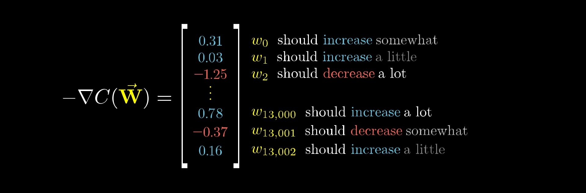
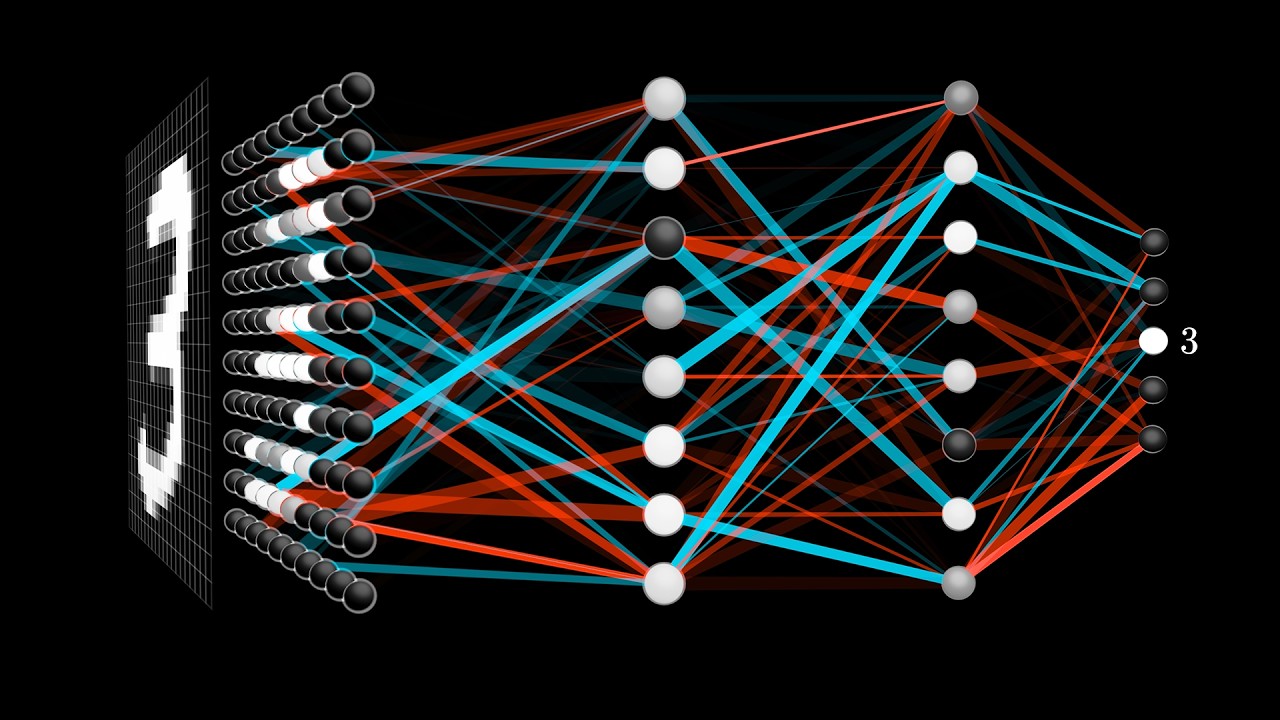
You see, in our network, an adjustment to one weight might have a greater impact on the cost function than an adjustment to some other weight. Consider the image below, and suppose that the network is supposed to be classifying its input as a "3".

Some weights have a larger impact on the cost than others.
Some of these connections just matter more for our training data than others, and a way you can think about the gradient of our massive cost function is that it encodes the relative importance of each weight and bias. That is, which changes will carry the most bang for your buck.
So if the cost function is a layer of complexity on top of the original neural network function, its gradient is one more layer of complexity still, telling us what nudge to all these weights and biases causes the fastest change to the value of the cost function.

The negative gradient tells us how to change the weights and biases to decrease the cost most effectively.
The algorithm for computing the value of this gradient vector efficiently is called backpropagation, which we'll dig into in the next lesson. There, I want to take the time to really walk through what happens to each weight and bias for a given piece of training data, trying to give an intuitive feel for what's happening beyond the pile of relevant formulas.
The main thing I want you to understand here, independent of implementation details, is that when we refer to a network "learning", we mean changing the weights and biases to minimize a cost function, which improves the network's performance on the training data.
But before we continue on to learn the details of computing this gradient, let's take a to dig into what this network looks like after it's trained.

Thanks
Special thanks to those below for supporting this lesson.