Chapter 3Analyzing our neural network

In the last post, we learned about how training a neural network involves minimizing a cost function with gradient descent. In the next post, we’ll dig into how the relevant gradient is computed. But before that, as a brief interlude, I want to skip ahead and have you look at what the result of this whole process is.

This entire mini lesson will be all about analyzing the trained neural network to see exactly what it does and why. But before you do any reading, it’s good to get your hands messy and try to discover for yourself exactly what this network is up to.

That’s why we’re bringing back the digit drawing demo from the very first lesson. But this time, to aid in your experimentation, all the neurons update live as you’re drawing, so you can get an immediate sense of how the input pixels affect the hidden layers and eventually the output.

Spend a bit of time experimenting, now with a bit more knowledge of how this whole system actually works, and then we’ll discuss what’s going on.

Analyzing the Network

The network we’ve developed, with two hidden layers of 16 neurons each, chosen mostly for aesthetic reasons, is… not bad. It classifies about 96% of new images it sees correctly. And honestly, if you look at some of the examples it messes up on, you feel compelled to cut it a little slack.

If you play around with the hidden layer structure and make some tweaks, you can get this up to about 98%. That’s pretty good! Although it’s not the best. Modern neural networks, which add in more sophisticated ideas than our plain vanilla variant, can have testing accuracy as high as 99.75%.¹ And frankly, looking through the MNIST database, I’m not even sure if most humans could do better than that.

Given how daunting the initial task is, there’s something incredible about any network doing this well on images it’s never seen, given that we never specifically told it what patterns to look for.

What Are These Layers Doing?

Originally, I motivated this layer structure by describing a hope that the second layer might pick up on little edges, while the third layer picks up on the subcomponents that form a digit. So, is this what our network has actually learned to do?

Well, for this one at least, not at all! Remember how in the first lesson, I said the weights leading to a given neuron in the second layer can be visualized as a pixel pattern that the second layer neuron is picking up on?

When we look at the weights associated with the transition from the first layer to the next, instead of picking up on isolated little edges here and there, they look, well, almost random. There are some loose patterns, but hardly the ones we might expect.

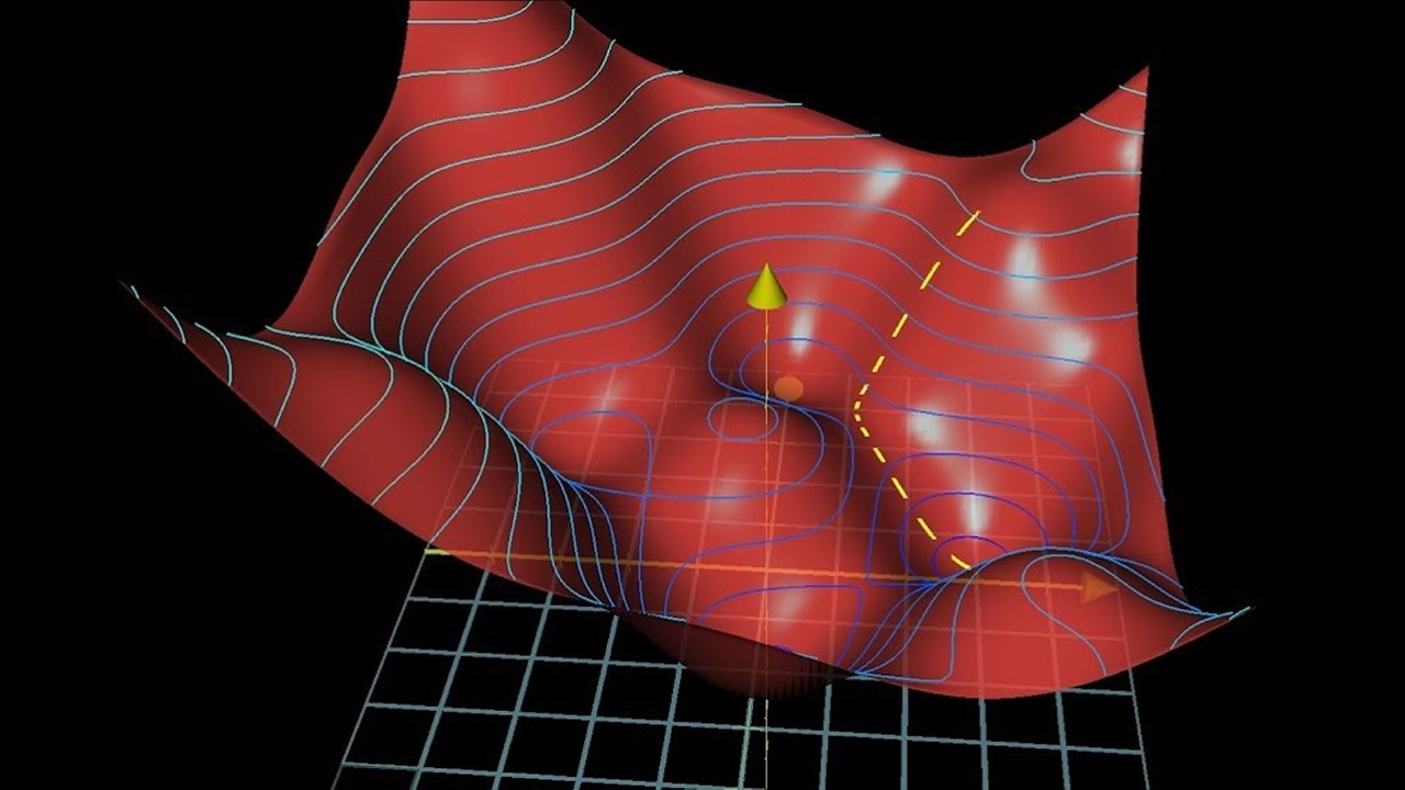
It seems that in the unfathomably large 13,002-dimensional space of possible weights and biases, the network found itself a happy little local minimum that, despite successfully classifying most images, doesn’t exactly pick up on more generalizable patterns.

To really drive this point home, watch what happens when you input a random image:

If the system was intelligent, you might expect it to feel really uncertain, either not really activating any of those ten output neurons or activating them all evenly. Instead, it confidently gives some nonsense answer, as if it feels as sure that this random noise is a 5 as it does that an actual image of a 5 is a 5.

This suggests that even if this network can recognize digits, it has no idea how to draw them.

Much of this is because it’s such a tightly constrained training setup. From the network’s point of view, the entire universe consists of nothing but clearly defined unmoving digits centered on a tiny grid, and its cost function never gave it an incentive to be anything but utterly confident in its decisions.

You might wonder why I’d introduce this network with the motivation of picking up on edges and patterns when that’s not at all what it ends up doing. Well, this is not meant to be an end goal, but instead a starting point.

Frankly, this is old technology, the kind researched in the ‘80s and ‘90s. You need to understand this before getting to more detailed modern variants, and it clearly is capable of solving some interesting problems! But the more you dig into what’s going on in these hidden layers, the less intelligent it seems.

Let’s return to the drawing demo. These 2nd layer weight grids, which aren’t really picking up on the edges we hoped for, but instead on some strange blobby shapes, are visible within the demo if you click on any neuron in the 2nd layer.

What’s even cooler is that if you’re looking at the weight grid for a particular neuron while drawing a digit, you can watch the weights be “revealed”, which changes the value of the neuron.

One fun challenge is to try drawing a 3, and then slowly extending it so it becomes an 8. At some point the network’s prediction will change, and as that’s happening, watch for which neuron(s) in the 2nd layer are changing, and then to figure out why they change as the 3 becomes an 8.

As you spend time playing with the network, you’ll start to find all kinds of edge cases where it gets confused or gives the wrong answer or just behaves in a way that isn’t as intelligent as we might hope. This technology is cool, but it isn’t perfect.

Again, think about what a constrained training environment this network had. Every digit that it saw was of a particular size, centered in the frame. So if you give it something that is too big or too small or not quite in the center, it is bound to get confused.

Our current learning algorithm does nothing to let the network transfer knowledge of patterns picked up on one region of the grid to another, or to make inferences about scaling. In fact, nothing about our training algorithm even uses the fact that some pixels are adjacent to others.

If you start thinking hard about how to change structure of this network to allow for more flexible learning, e.g. how learning a pattern in one part of the image could naturally transfer to any other part of the image, you’ll be well situated to learn about some of the more modern variations on this theme, most notably convolutional neural networks.

But we’re getting ahead of ourselves. Before that, it’s time to learn about backpropagation, the workhorse behind neural network training.