But what is a Fourier series? From heat flow to circle drawings
How Fourier series arose from studying heat flow, and how they can be thought of as decomposing any drawing in 2d into a sum of rotations.
Intro
Here, we look at the math behind an animation like this, what's known as a "complex Fourier series".
Each little vector is rotating at some constant integer frequency, and when you add them all together, tip to tail, they draw out some shape over time. By tweaking the initial size and angle of each vector, we can make it draw anything we want, and here you'll see how.
Before diving in, take a moment to linger on just how striking this is. Go full screen for this if you can, the intricacy is worth it.
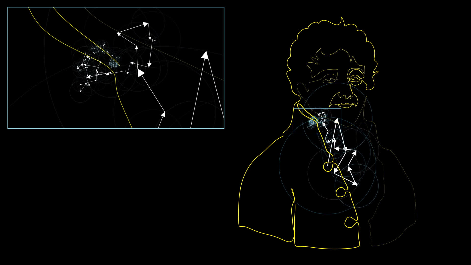
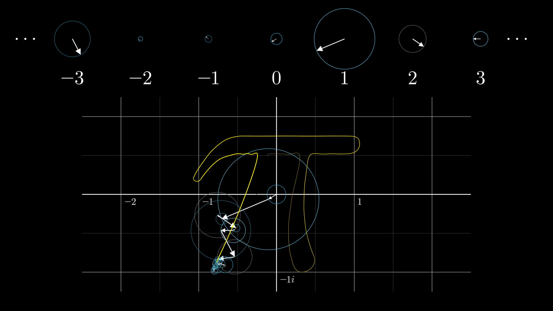
A single-line portrait of Joseph Fourier, as drawn by a Fourier series.
How many rotating arrows would you guess are used in the animation above to draw a picture of Joseph Fourier?
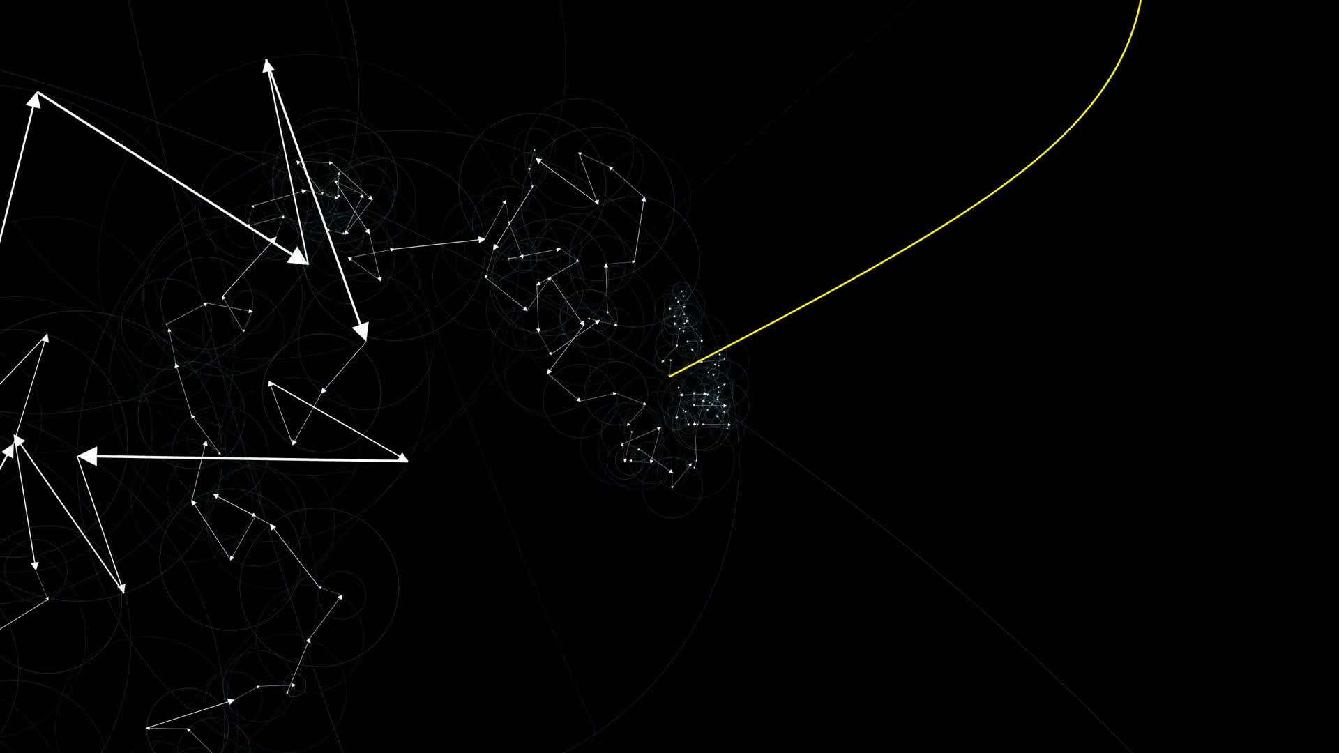
Think about this, the action of each individual arrow is perhaps the simplest thing you could imagine: Rotation at a steady rate. Yet the collection of all added together is anything but simple. The mind-boggling complexity is put into even sharper focus the farther we zoom in, revealing the contributions of the littlest, quickest arrows.
Considering the chaotic frenzy you're looking at, and the clockwork rigidity of the underlying motions, it's bizarre how the swarm acts with a kind of coordination to trace out some very specific shape. Unlike much of the emergent complexity you find elsewhere in nature, though, this is something we have the math to describe and to control completely. Just by tuning the starting conditions, nothing more, you can make this swarm conspire in all the right ways to draw anything you want, provided you have enough little arrows. What's even crazier, as you'll see, is the ultimate formula for all this is incredibly short.
c_n = \int_0^1 e^{-2 \pi i n \cdot t} f(t) dtWe'll explain what this expression means and how to read it in just a bit.
Often, Fourier series are described in terms of functions of real numbers being broken down as a sum of sine waves. That turns out to be a special case of this more general rotating vector phenomenon that we'll build up to, but it's where Fourier himself started, and there's good reason for us to start the story there as well.
Already, a coupld questions might come to mind. What does adding sine waves have to do with the circle animations? And perhaps more pertinantly, why would anyone care? What problems does this solve?
Technically, this is the third lesson in a , which Fourier was working on when he developed his big idea. I'd like to teach you about Fourier series in a way that doesn't depend on you coming from those chapters, but if you have at least a high-level idea of the problem from physics which originally motivated this piece of math, it gives some indication for how unexpectedly far-reaching Fourier series are.
If you don't care about the historical and physics-based origins of this math, or if you're coming from the previous chapters, feel free to skip the next few sections. If you do care, or you want a quick recap, let's dive on in.
The heat equation (recap)
Suppose you have some object, which for simplicity we'll think of as being one-dimensional, like a rod, and you know the temperature at every point on this rod at a given snapshot in time, which we'll call t = 0.
We'll call this the initial temperature distribution on the rod.
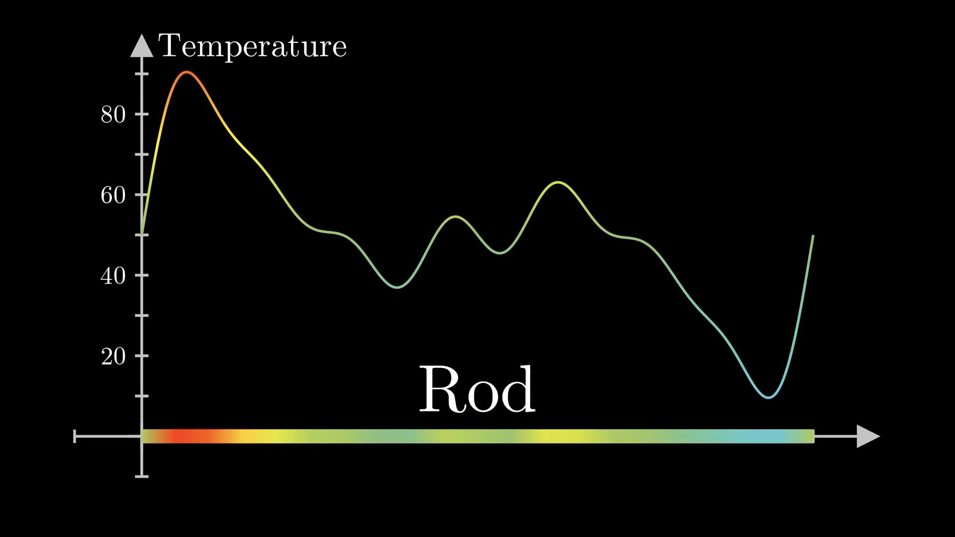
As time ticks forward, the hot points will tend to cool down, and the cold points will tend to warm up, with an all around tendency for a more even temperature distribution. How quickly this happens is determined by a constant \alpha, known as the thermal diffusivity, which depends on the material. But how specifically the shape of this distribution changes over time is determined by what's known as the heat equation.
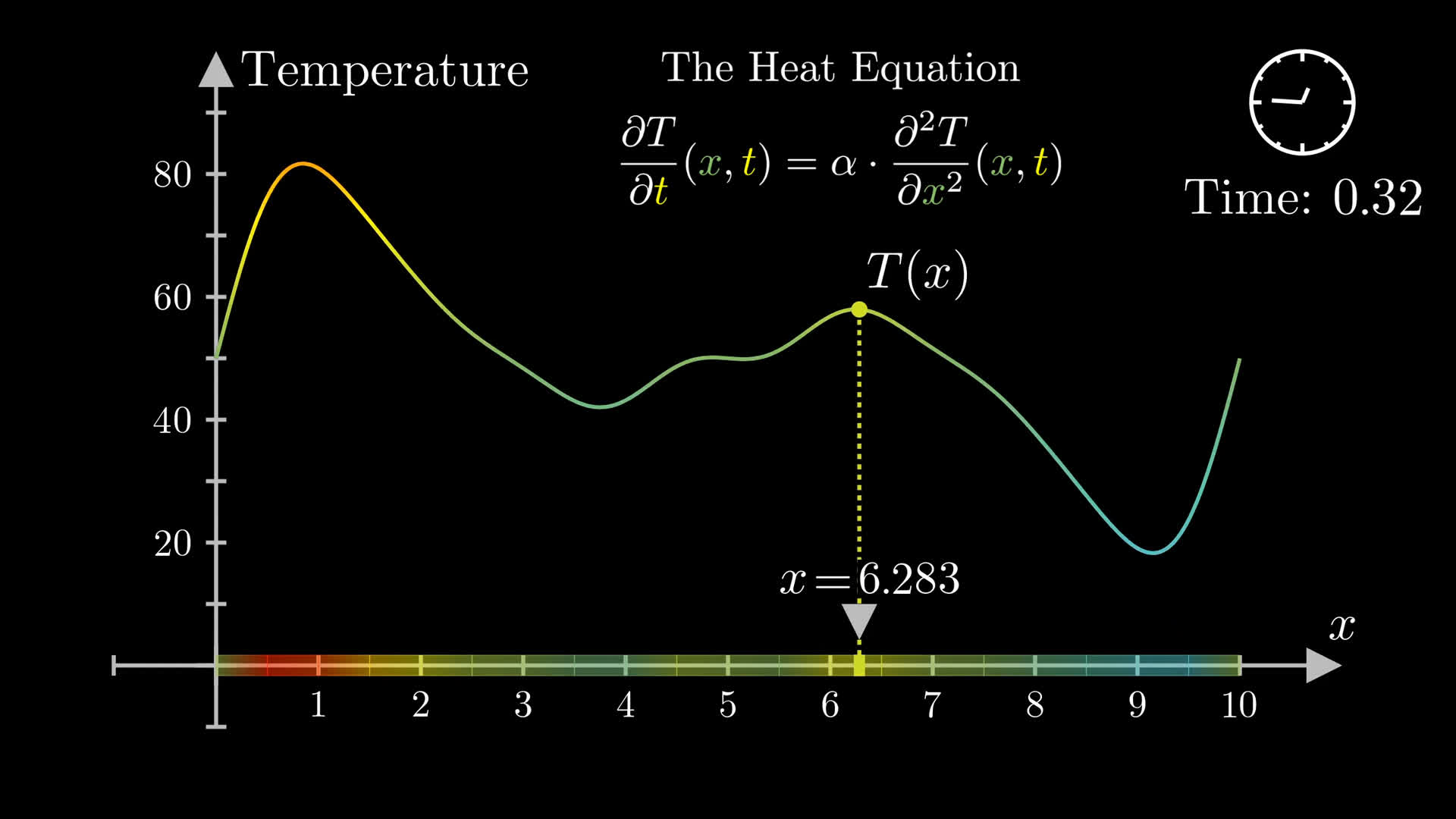
The heat equation is a partial differential equation, which the lessons describe in much more detail. For now all you need to know is that it does not directly tell you what future distributions will look like. Instead, together with an initial distribution and some condition on the boundary of the rod, it gives a constraint that this evolution of future distribution must satisfy. It is up to the mathematician to actually solve this equation if they want a specific formula for how the temperature is distributed at any time t > 0.
Enter Fourier.
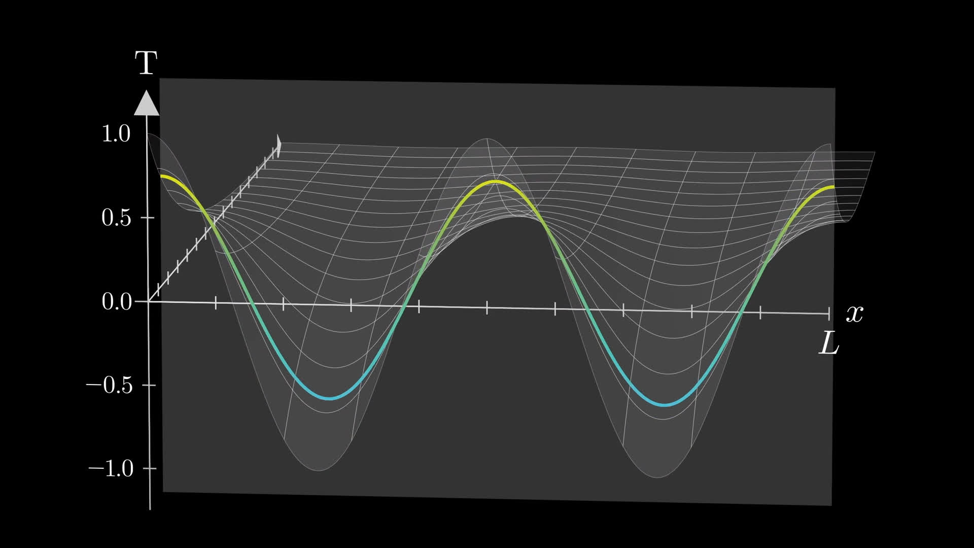
While it's exceedingly challenging to directly to directly solve this equation for a given initial distribution, there's a simple solution if that initial function happens to look like a cosine wave with a frequency tuned to make it flat at each endpoint. Specifically, as you graph what happens over time, these waves simply get scaled down exponentially, with higher frequency waves decaying faster.
The heat equation happens to be what's known in the business as a "linear" equation, meaning if you know two solutions and you add them up, that sum is also a new solution. You can even scale them each by some constant, which gives you some dials to turn to construct a custom function solving the equation.
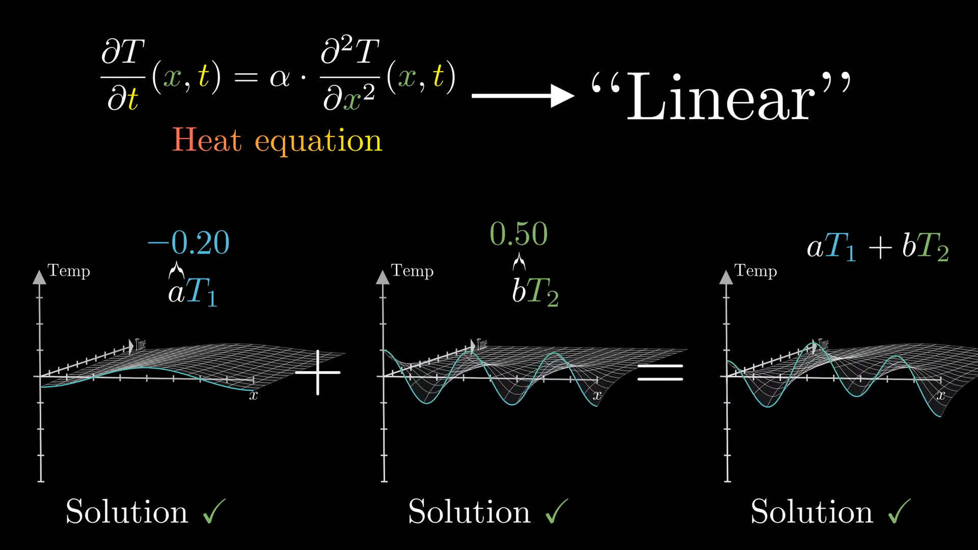
So even though it would be absurd to find a rod whose initial temperature distribution is a perfect cosine wave, this means we know how to solve the equation for a much bigger class of functions, anything which can be written as a scaled sum of waves. You solve the equation for each of those waves separately, then add them together.
It's hard to overstate how powerful this kind of linearity is. It means we can take our infinite family of solutions, these exponentially decaying cosine waves, scale a few of them by some custom constants of our choosing, and combine them to get a solution for a new tailor-made initial condition which is some combination of cosine waves. Linearity is the difference between having a scattered set of haphazard solutions in isolated cases, and having a massive space of solutions with knobs and dials to adjust that tune this initial condition to our liking.
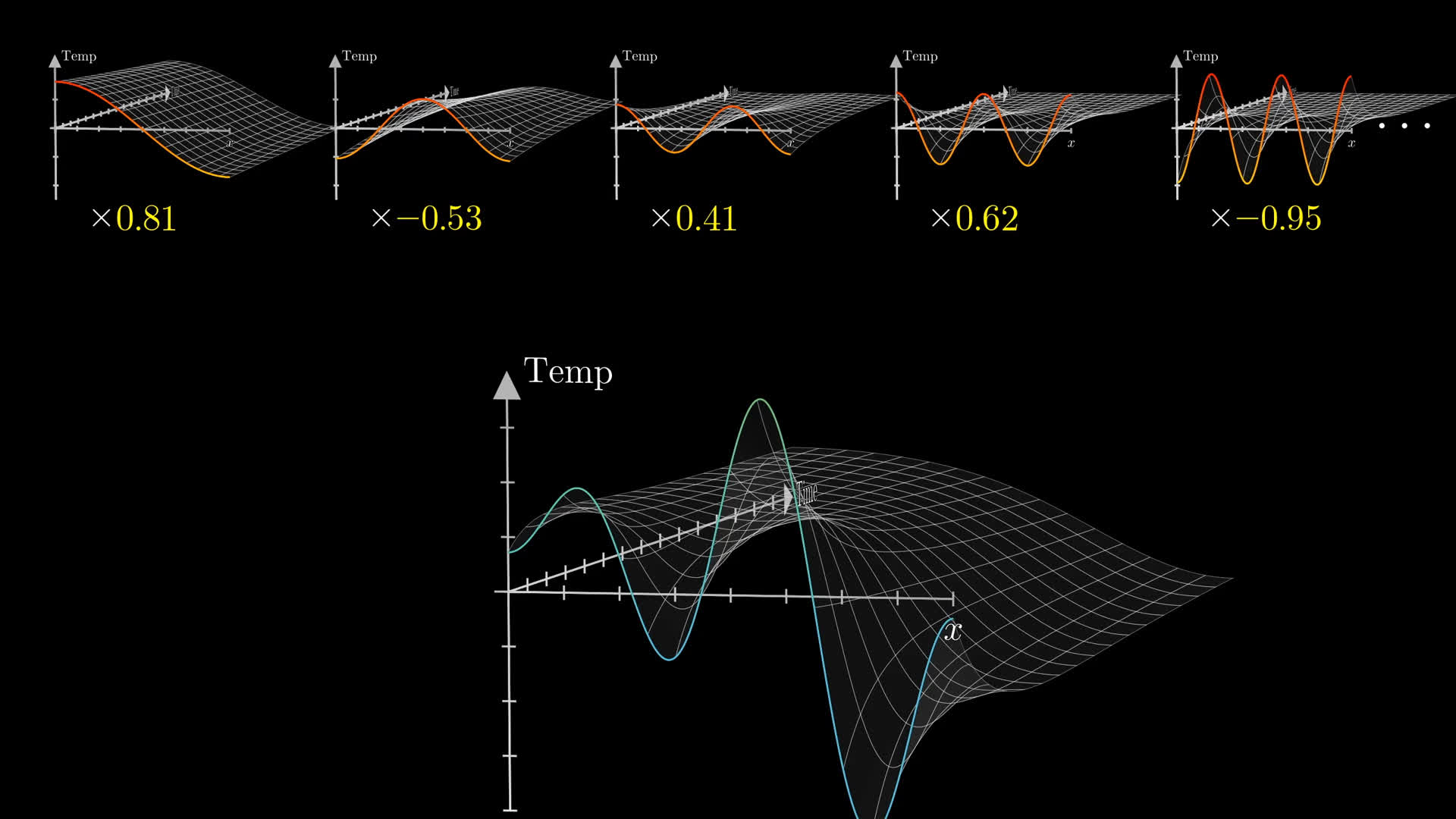
Something important I want you to notice about combining the waves like this is that because higher frequency ones decay faster, this sum which you construct will smooth out over time as the high-frequency terms quickly go to zero, leaving only the low-frequency terms dominating. So in some sense, all the complexity in the evolution that the heat equation implies is captured by this difference in decay rates for the different frequency components.
Fourier series
It's at this point that Fourier gains immortality. I think most normal people at this stage would say "well, I can solve the heat equation when the initial temperature distribution happens to look like a wave, or a sum of waves, but what a shame that most real-world distributions don't at all look like this!"
For example, let's say you brought together two rods, each at some uniform temperature, and you wanted to know what happens immediately after they come into contact. To make the numbers simple, let's say the temperature of the left rod is 1^{\circ}, and the right rod is -1^{\circ}, and that the total length L of the combined rod is 1.
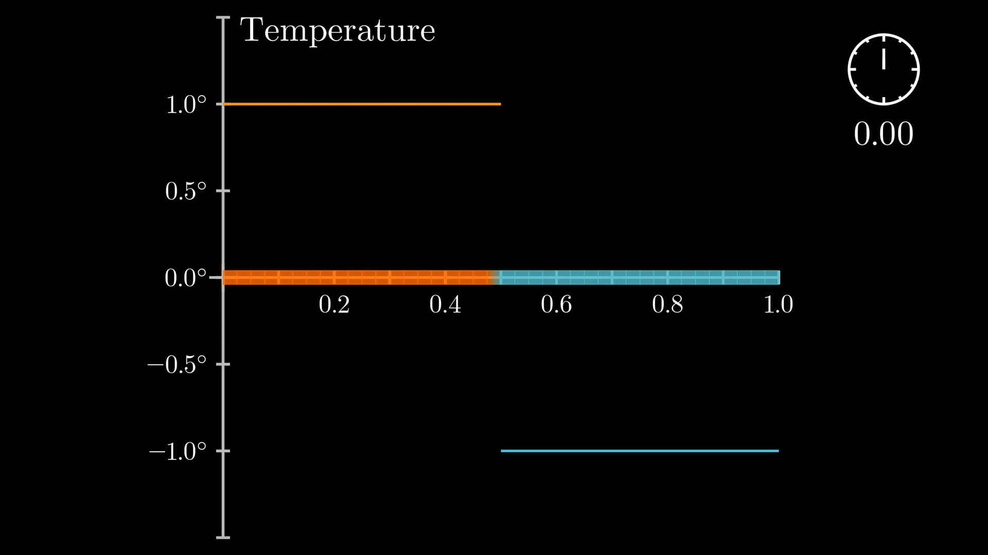
Our initial temperature distribution is a step function, which is so obviously different from sine waves and sums of sine waves, don't you think? It's almost entirely flat, not wavy, and for god's sake, it's even discontinuous!
And yet, Fourier thought to ask a question which seems absurd: How do you express this as a sum of sine waves? Even more boldly, how do you express any initial temperature distribution as a sum of sine waves?
And it's more constrained than just that! You have to restrict yourself to adding waves which satisfy a certain boundary condition, which as we saw in the last lesson means working only with these cosine functions whose frequencies are all some whole number multiple of a given base frequency.
Non-mathematical interlude
It's strange how often progress in math looks like asking a new question, rather than simply answering an old one.
Fourier really does have a kind of immortality, with his name essentially synonymous with the idea of breaking down functions and patterns as combinations of simple oscillations.
Fourier could never have imagined how significant and far-reaching this idea would turn out to be, ranging from the study of prime numbers, to quantum computing, to signal processing and much more. And yet, the origin of all this is in a piece of physics which upon first glance has nothing to do with frequencies and oscillations.
Infinite sinusoids?
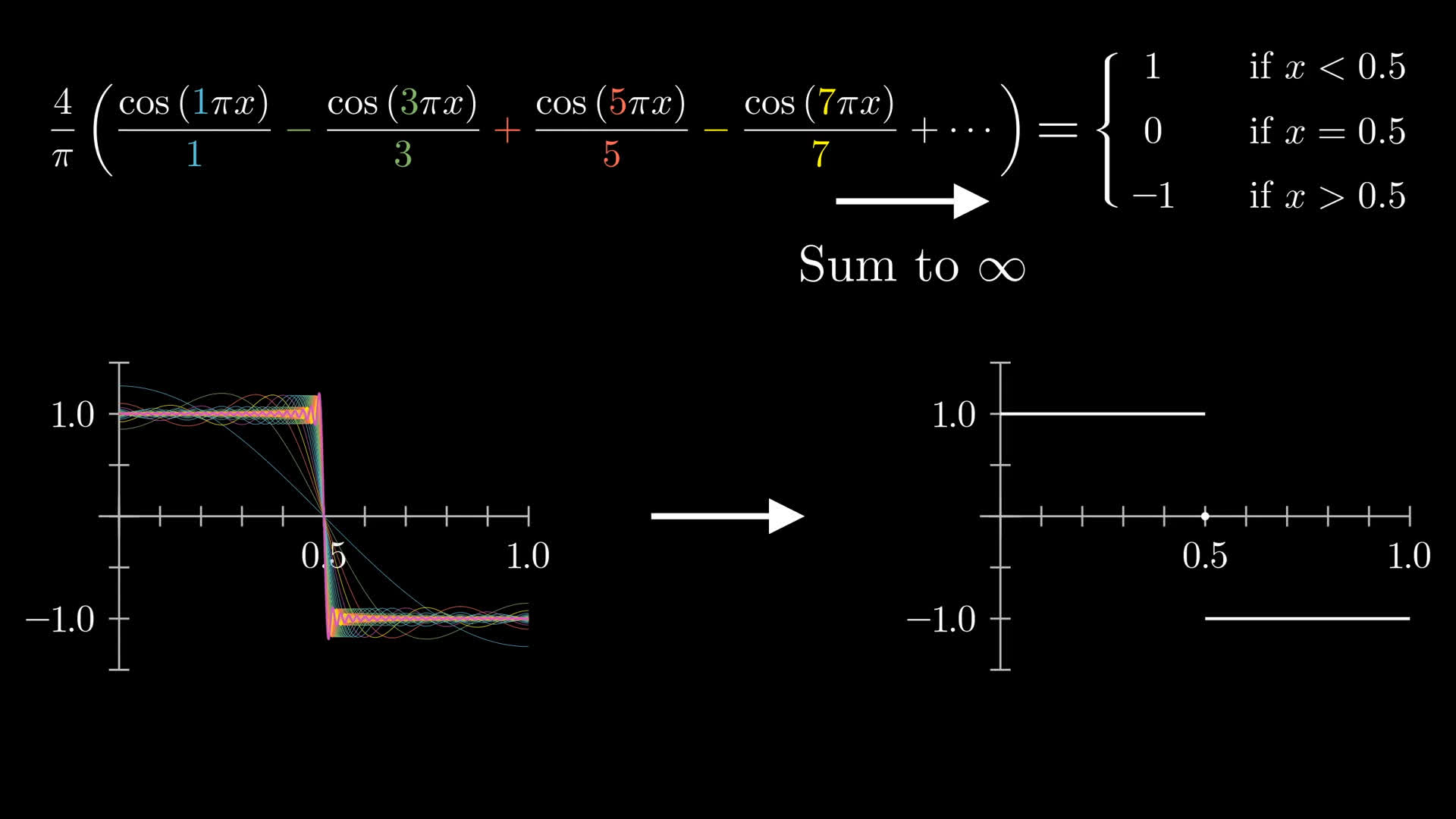
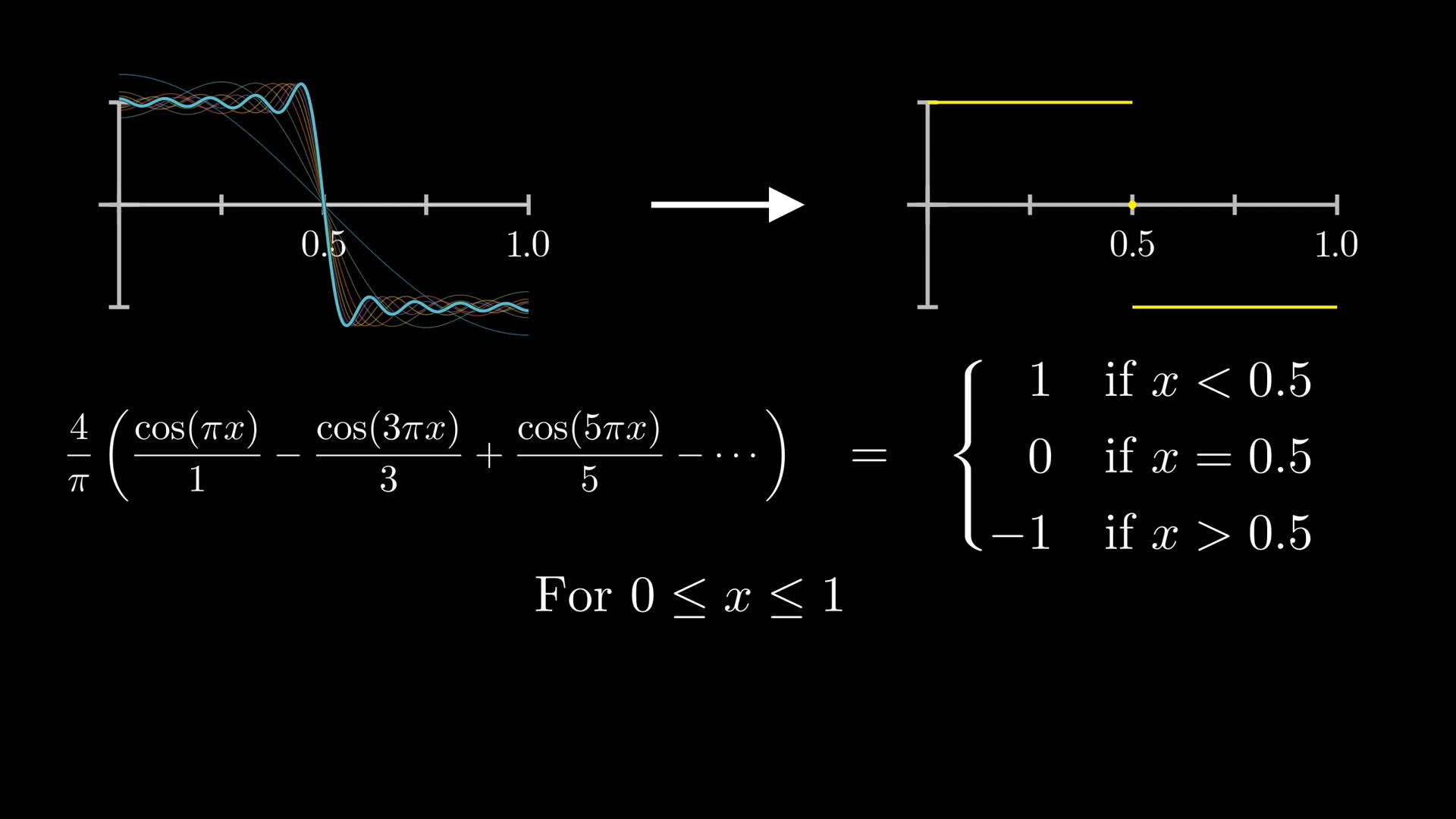
"Now hang on," I hear some of you saying, "none of these sums of sine waves being shown are actually the step function." It's true, any finite sum of sine waves will never be perfectly flat (except for a constant function), nor discontinuous. But Fourier thought more broadly, considering infinite sums. In the case of our step function, it turns out to be equal to this infinite sum:
2 \cdot H(x - 0.5) - 1 = \frac{4}{\pi} \left( \frac{\cos(1 \pi x)}{1} - \frac{\cos(3 \pi x)}{3} + \frac{\cos(5 \pi x)}{5} - \frac{\cos(7 \pi x)}{7} + \cdots \right)I'll explain where these numbers come from in a moment.
Before that, it's worth being clear about what we mean with a phrase like "infinite sum", which runs the risk of being vague. Consider the simpler context of adding numbers, say this alternating sum of fractions with odd denominators:
\frac{1}{1} - \frac{1}{3} + \frac{1}{5} - \frac{1}{7} + \frac{1}{9} - \frac{1}{11} \cdots = \frac{\pi}{4}If you add these terms successively, one-by-one, at all times what you have will be rational. At no point will your partial sum of N terms equal the irrational \frac{\pi}{4}. But this sequence of partial sums approaches \frac{\pi}{4}. The numbers you see get arbitrarily close to that value, and stay arbitrarily close to that value.
Referencing partial sums, and what that sequence of values approaches, is all a bit of mouthful, so instead we abbreviate and say the infinite sum "equals" \frac{\pi}{4}.
With functions, you're doing the same thing but with many different values in parallel. Consider a specific input, like x=0.2, and the value of all these scaled cosine functions for that input.
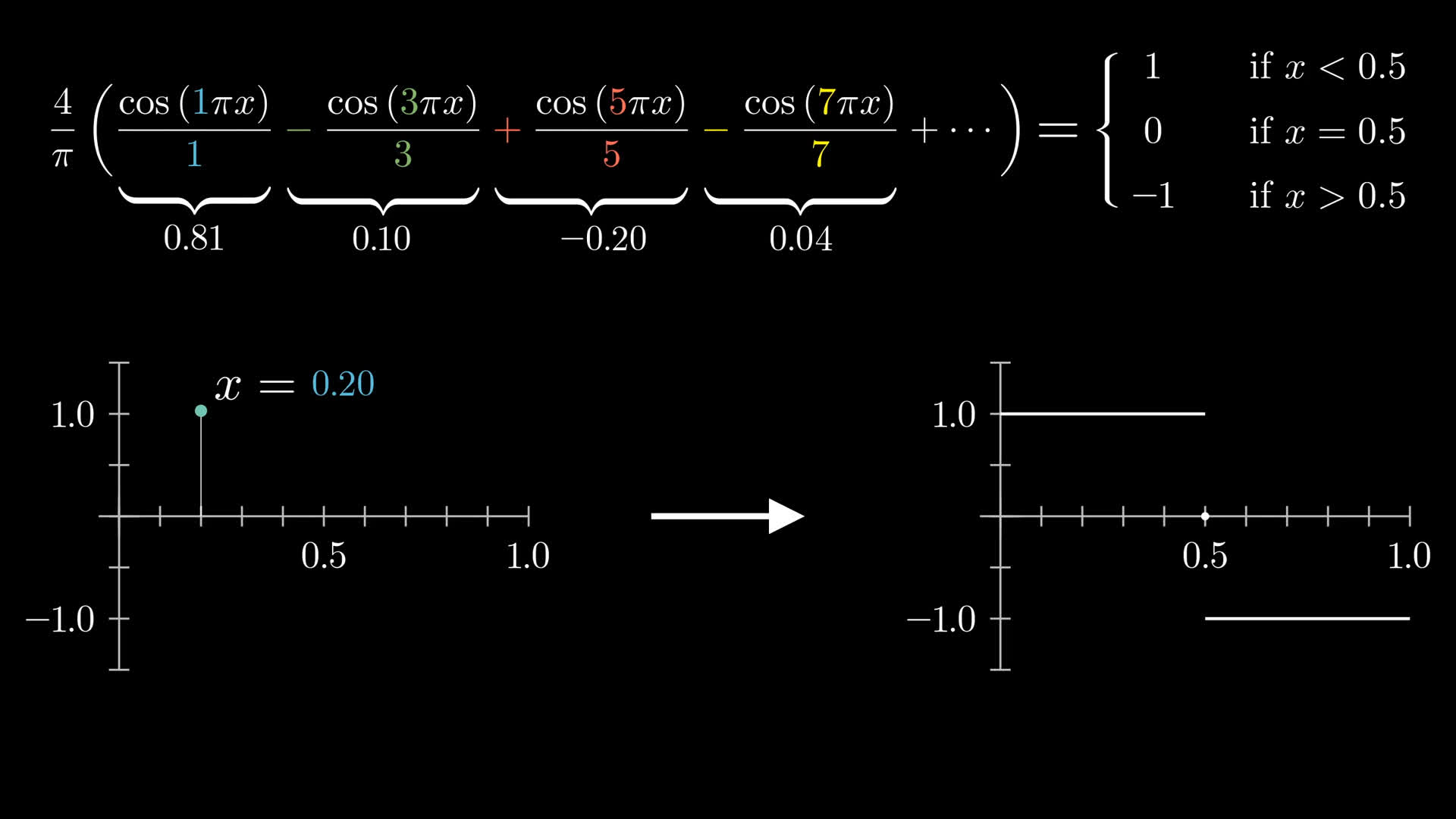
If that input is less than 0.5, as you add more and more terms, the sum will approach 1.
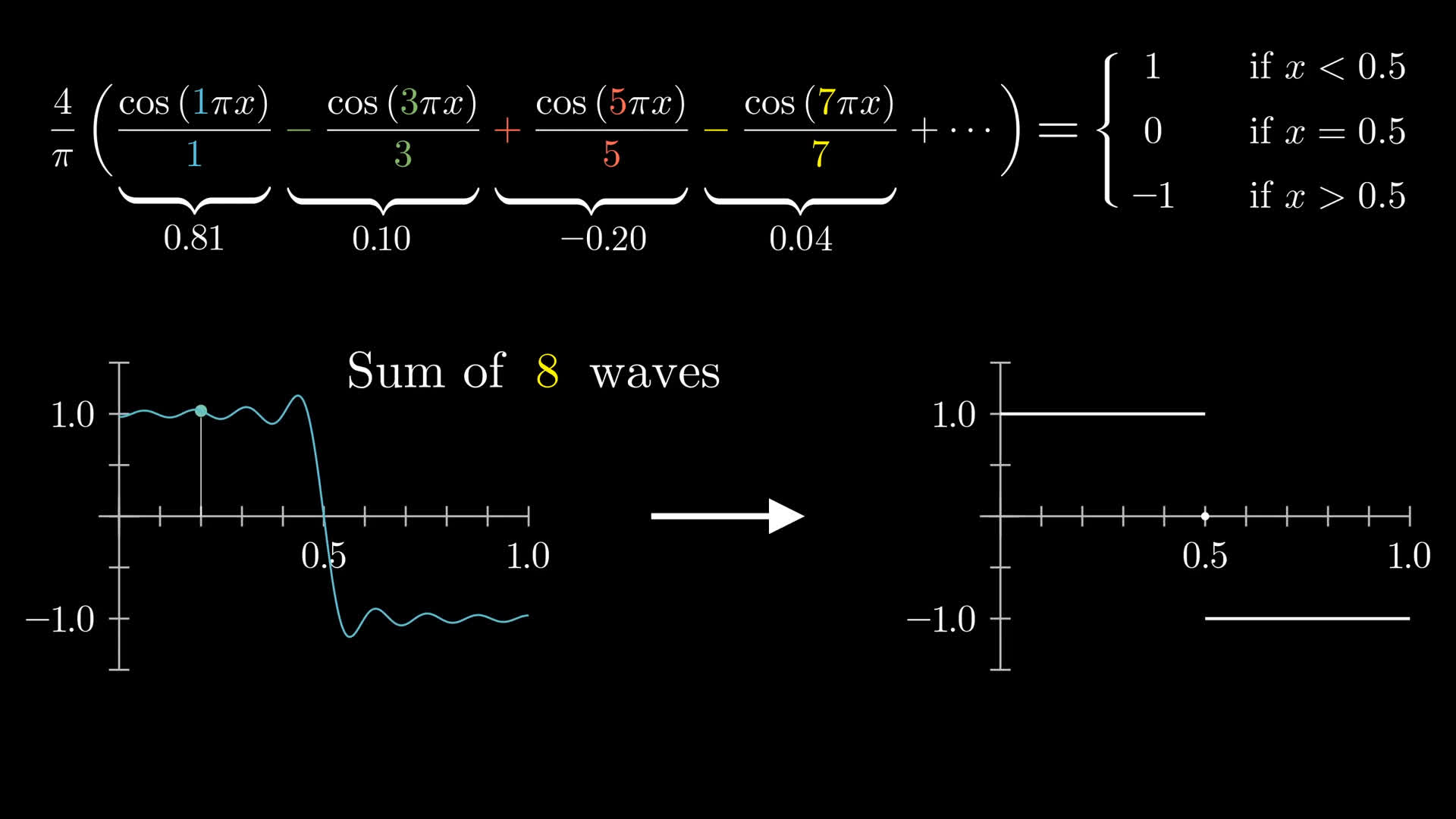
If that input is greater than 0.5, as you add more and more terms it would approach -1.
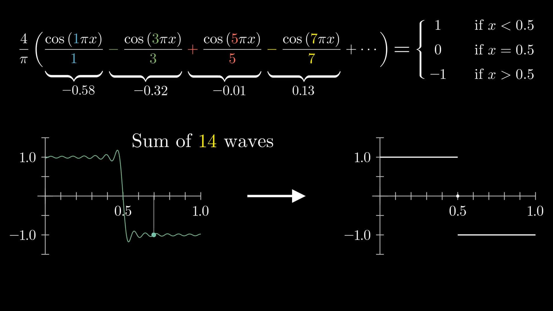
At the input 0.5 itself, all the cosines are 0, so the limit of the partial sums is 0.
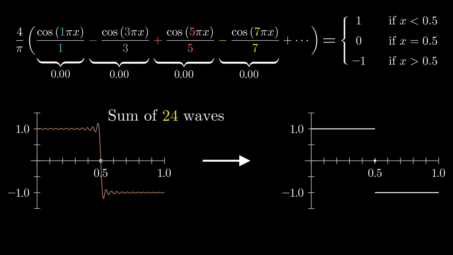
Somewhat awkwardly, then, for this infinite sum of functions to be strictly true, we do have to prescribe the value of the step function at the point of discontinuity to be 0.
Analogous to an infinite sum of rational numbers being irrational, the infinite sum of wavy continuous functions can equal a discontinuous flat function. Limits allow for qualitative changes which finite sums alone never could.
There are multiple technical nuances I'm sweeping under the rug here.
- Does the fact that we're forced into a certain value for the step function at its point of discontinuity make any difference for the heat flow problem?
- For that matter, what does it really mean to solve a PDE with a discontinuous initial condition?
- Can we be sure the limit of solutions to the heat equation is also a solution?
- Can all functions be expressed as an infinite sum of waves like this?
These are exactly the kind of questions real analysis is built to answer, but it falls a bit deeper in the weeds than I think we should go here.
The upshot is that when you take the heat equation solutions associated with these cosine waves and add them all up, all infinitely many of them, you do get an exact solution describing how the step function will evolve over time.
How do we compute the coefficients?
Generalize
The key challenge, of course, is to find these coefficients, the terms which we scale each wave by before adding them up. So far, we've been thinking about functions with real number outputs, but for the computations I'd like to show you something more general than what Fourier originally did, applying to functions whose output can be any complex number, which is where those rotating vectors from the opening come back into play.
Why the added complexity? Aside from being more general, in my view the computations become cleaner and it's easier to see why they work. More importantly, it sets a good foundation for ideas that will come up again later in the series, like the Laplace transform and the importance of exponential functions.
Waves and rotation
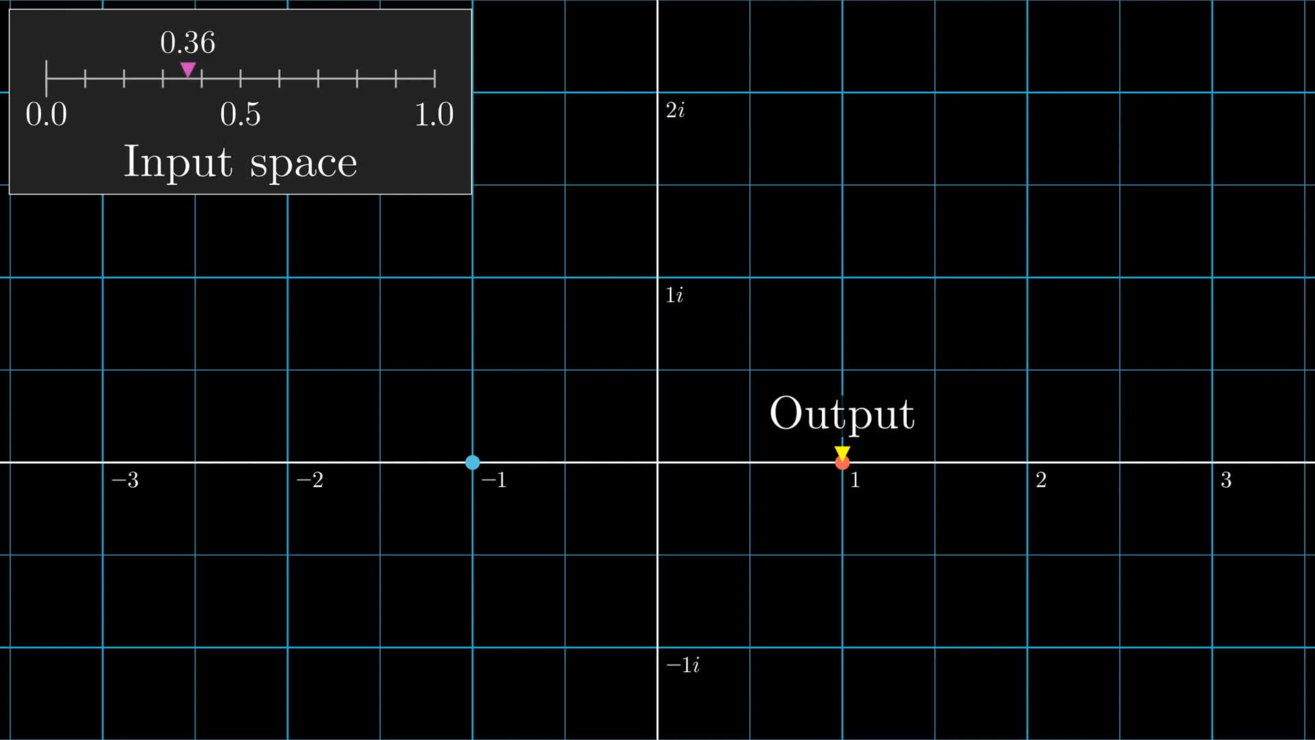
We'll still think of functions whose input is some real number on a finite interval, say the one from 0 to 1 for simplicity. But whereas something like a temperature function will have an output confined to the real number line, we'll broaden our view to outputs anywhere in the two-dimensional complex plane.
You might think of such a function as a drawing, with a pencil tip tracing along different points in the complex plane as the input ranges from 0 to 1.
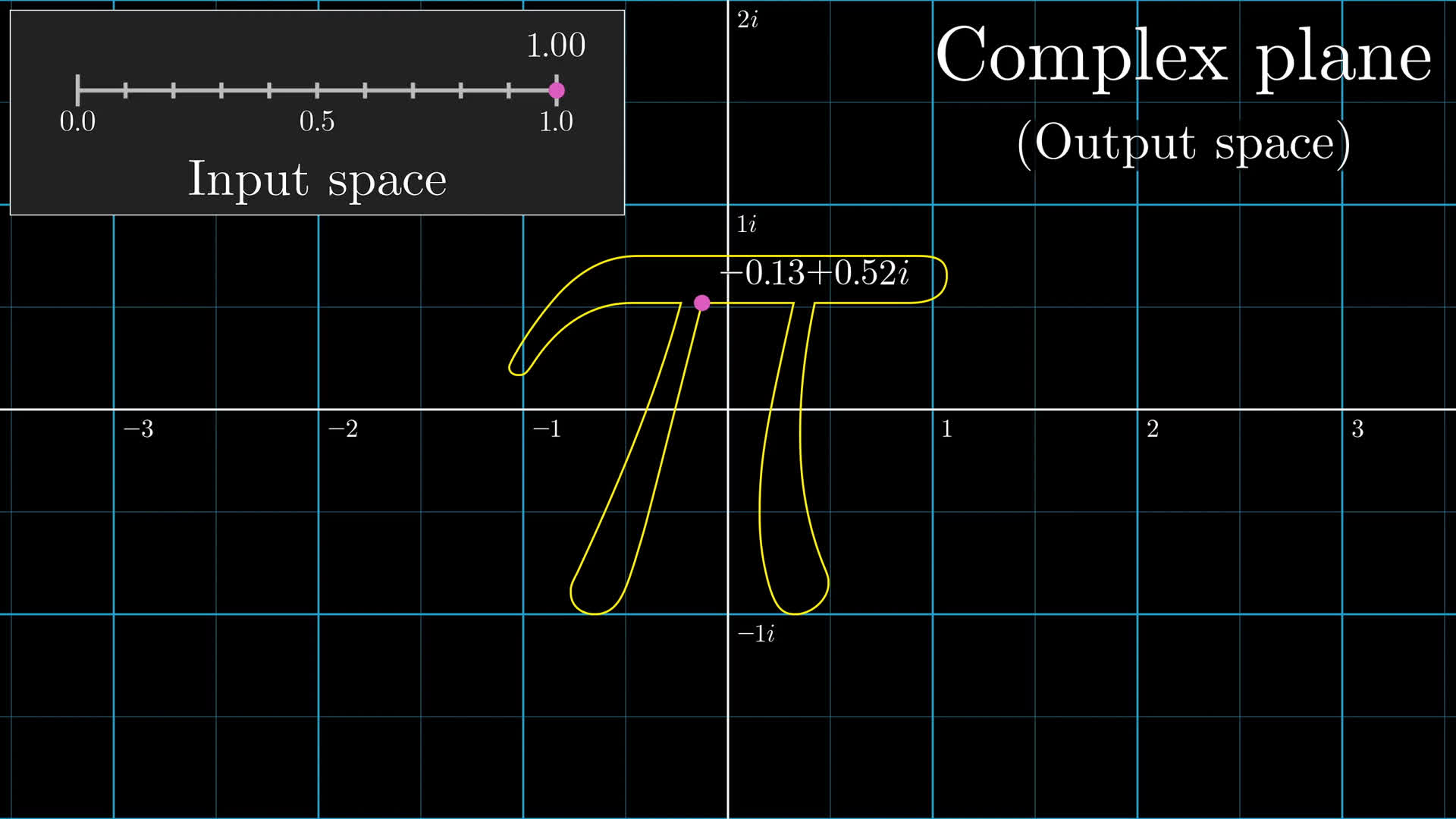
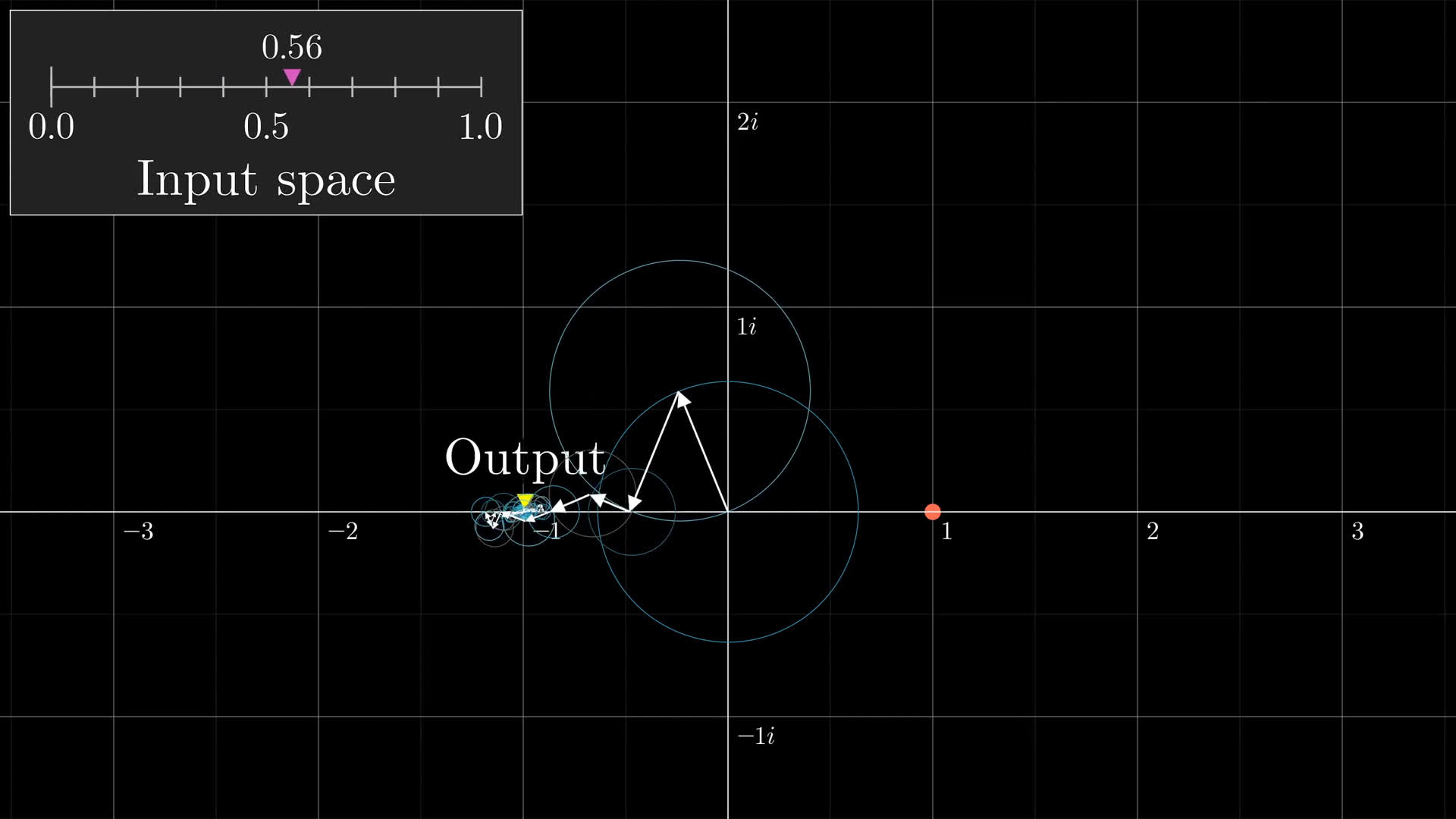
Instead of sine waves being the fundamental building block, we'll focus on breaking these functions down as a sum of little vectors, all rotating at some constant integer frequency.
Functions with real number outputs are essentially really boring drawings; a 1-dimensional pencil sketch confined to the real number line. You might not be used to thinking of them like this, since usually we visualize such a function with a graph, but right now the path being drawn is only in the output space.
When we do the decomposition into rotating vectors for these boring 1d drawings, what will happen is that all the vectors with frequency 1 and -1 will have the same length, and they'll be horizontal reflections of each other. When you just look at the sum of these two as they rotate, that sum stays fixed on the real number line, and oscillates like a sine wave.
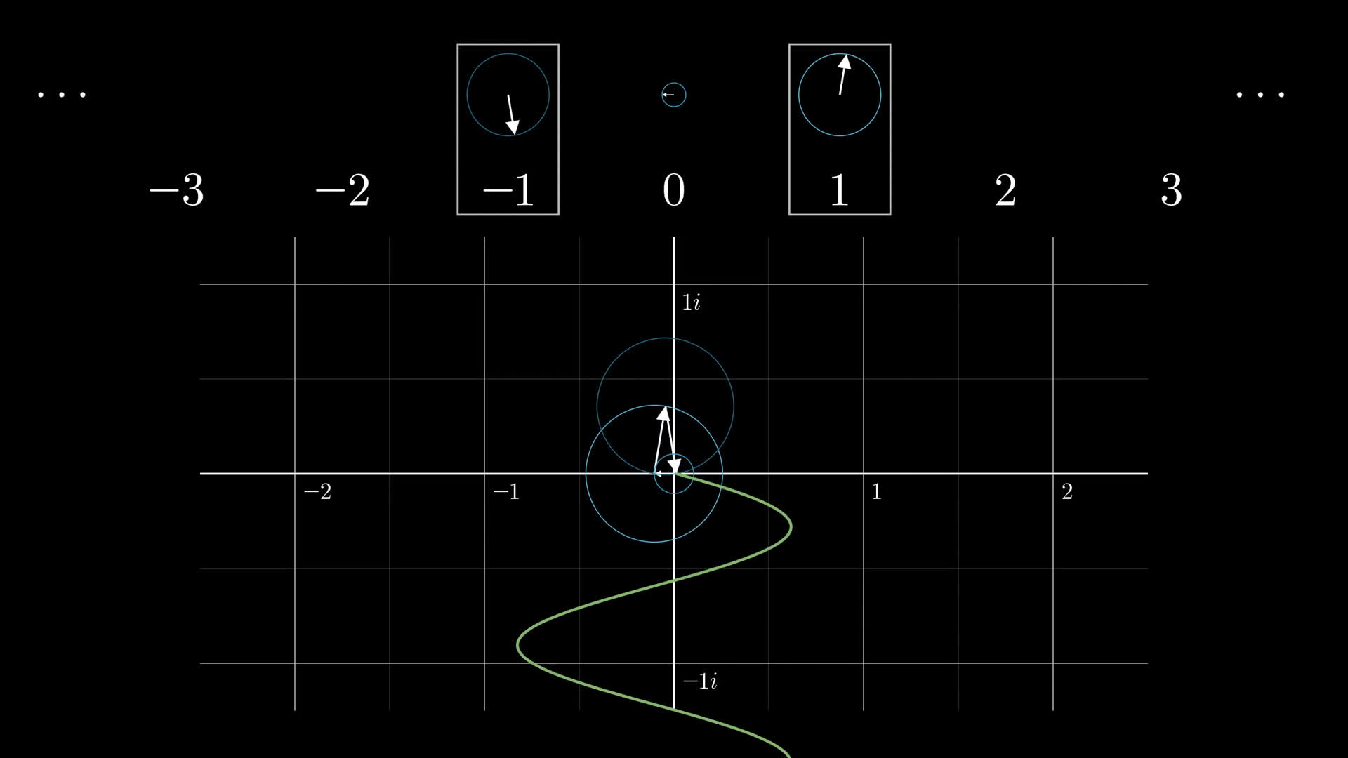
This might be a weird way to think about a sine wave, since we're used to looking at its graph rather than the output alone wandering on the real number line. But in the broader context of functions with complex number outputs, this is what sine waves look like. Similarly, the pair of rotating vectors with frequency 2, -2 will add another sine wave component, and so on, with the sine waves we were looking at earlier now corresponding to pairs of vectors rotating in opposite directions.
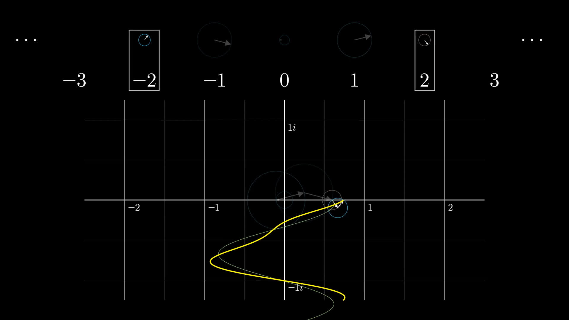
So the context Fourier originally studied, breaking down real-valued functions into sine wave components, is a special case of the more general idea with 2d-drawings and rotating vectors.
At this point, maybe you don't trust me that widening our view to complex functions makes things easier to understand, but bear with me. It really is worth the added effort to see the fuller picture, and I think you'll be pleased by how clean the actual computation is in this broader context.
Complex numbers
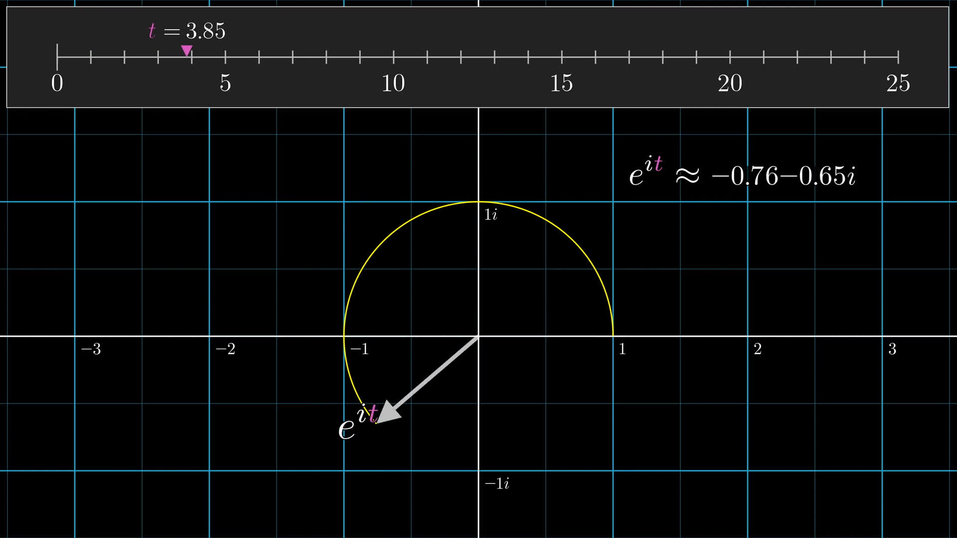
You may also wonder why, if we're going to bump things up to 2-dimensions, we don't we just talk about 2d vectors; What does \sqrt{-1} have to do with anything? Well, the heart and soul of Fourier series is the complex exponential, e^{it}. As the value of t ticks forward with time, this value walks around the unit circle at a rate of 1 unit per second.
In the , you'll see a quick intuition for why exponentiating imaginary numbers walks in circles like this from the perspective of differential equations, and beyond that, as the series progresses I hope to give you some sense for why complex exponentials are important.
You see, in theory, you could describe all of this Fourier series stuff purely in terms of vectors and never breathe a word of i. The formulas would become more convoluted, but beyond that, leaving out the function e^x would somehow no longer authentically reflect why this idea turns out to be so useful for solving differential equations.
The key feature of e^x is that it's a function whose derivative equals itself, which makes it a useful building block for describing functions whose derivatives depend on the function itself in more complicated ways.
For right now you can think of this e^{i t} as a notational shorthand to describe a rotating vector, but just keep in the back of your mind that it's more significant than a mere shorthand.
In fact, if the back of your mind has a little extra space, you can think about how the second derivative of this function is equal to -1 times itself, and how this might correspond to the negative sign showing up in the heat equation.
I'll be loose with language and use the words "vector" and "complex number" somewhat interchangeably, since thinking of complex numbers as little arrows makes the idea of adding many together clearer.
So, what are the constants?
Armed with the function e^{it}, let's write down a formula for each of these rotating vectors we're working with. For now, think of each of them as starting pointed one unit to right, at the number 1.
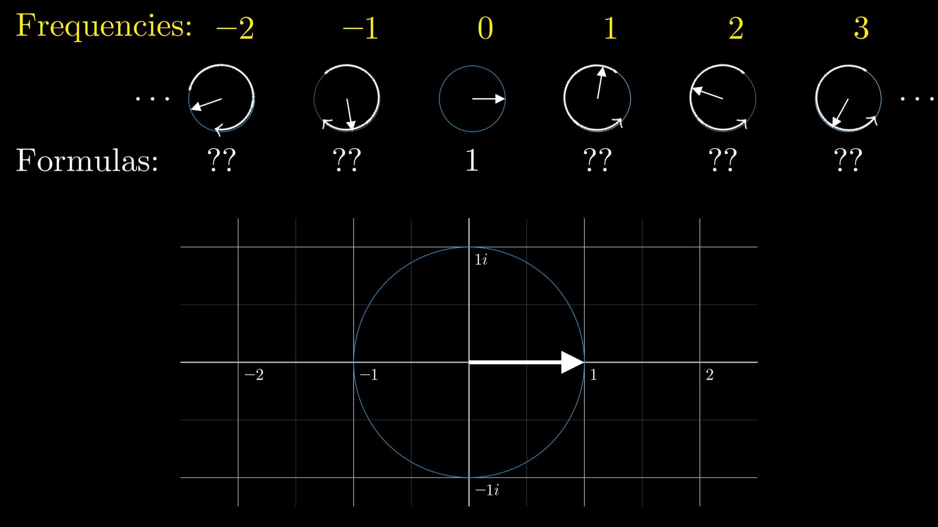
The easiest vector to describe is the constant one, which just stays at the number 1, never moving. Or, if you prefer, it's "rotating" at a frequency of 0.
Then there will be a vector rotating 1 cycle every second which we write as e^{2 \pi i t}.
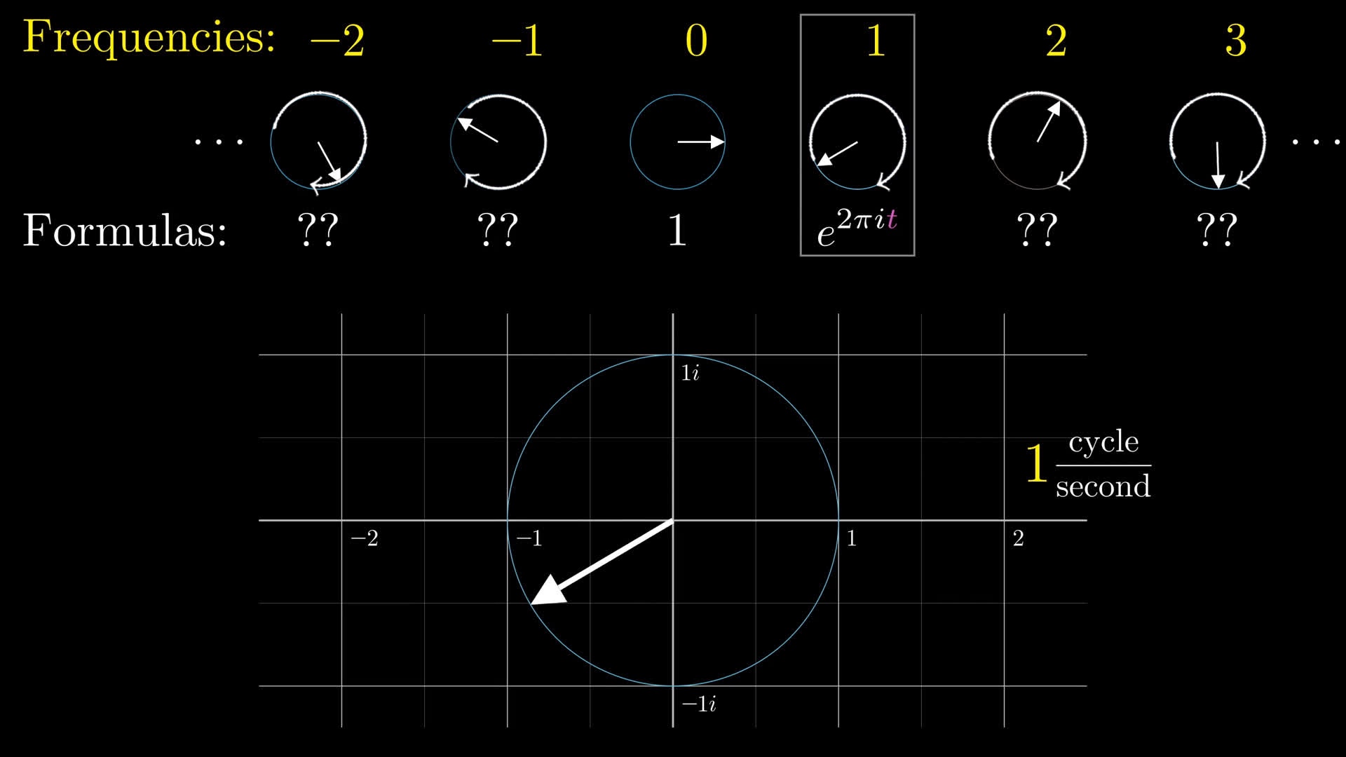
The 2 \pi is there because as t goes from 0 to 1, it needs to cover a distance of 2 \pi along the circle.
We also have a vector rotating at 1 cycle per second in the other direction, e^{-2 \pi i t}.
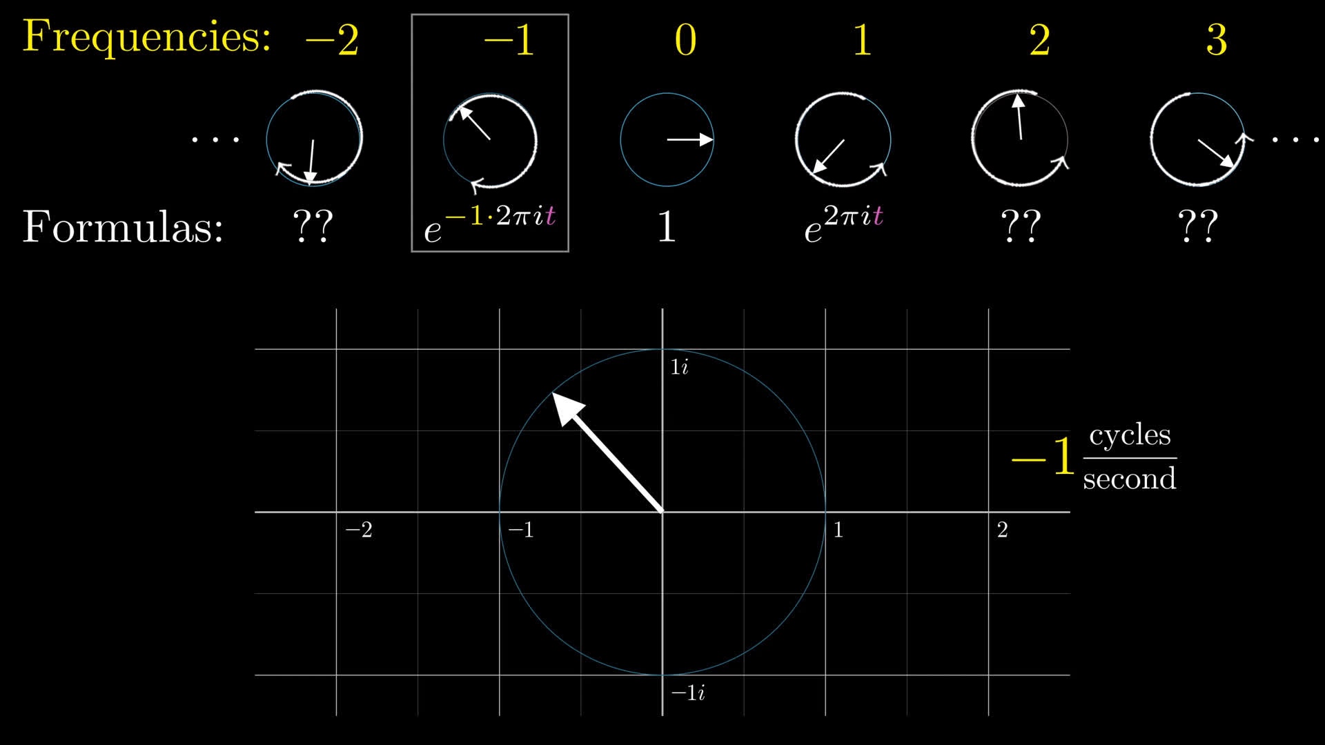
Similarly, the one going 2 rotations per second is e^{2 \cdot 2 \pi i t}, where that 2 \cdot 2 \pi in the exponent describes how much distance is covered in 1 second. And we go on like this over all integers, both positive and negative, with a general formula of e^{n \cdot 2 \pi i t} for each rotating vector.
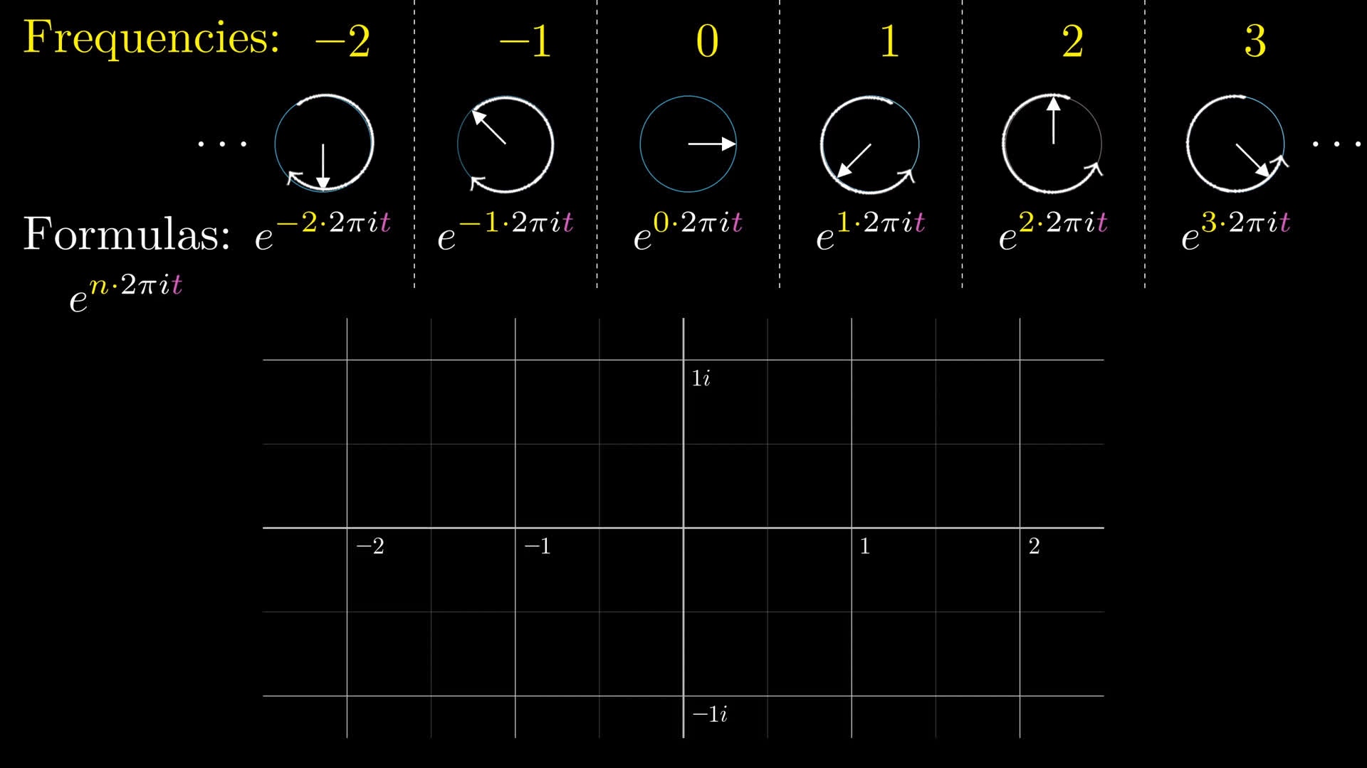
Notice, this makes it more consistent to write the constant vector is written as e^{0 \cdot 2 \pi i t}, which feels like an awfully complicated to write the number 1, but at least then it fits the pattern.
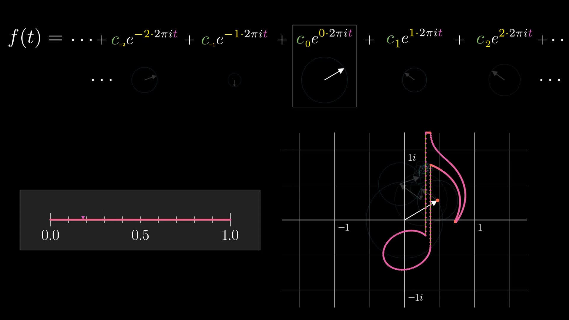
The control we have, the set of knobs and dials we get to turn, is the initial size and direction of each of these numbers. The way we control that is by multiplying each one by some complex number, which I'll call c_n.
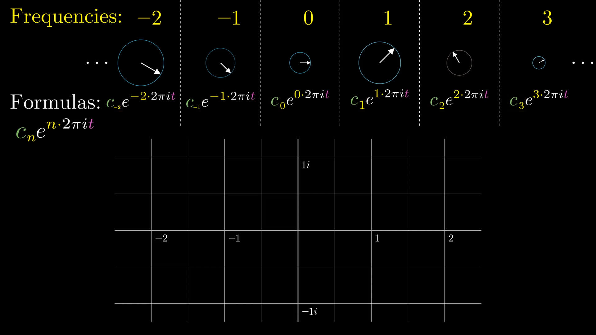
For example, if we wanted that constant vector not to be at the number 1, but to have a length of 0.5, we'd scale it by 0.5.
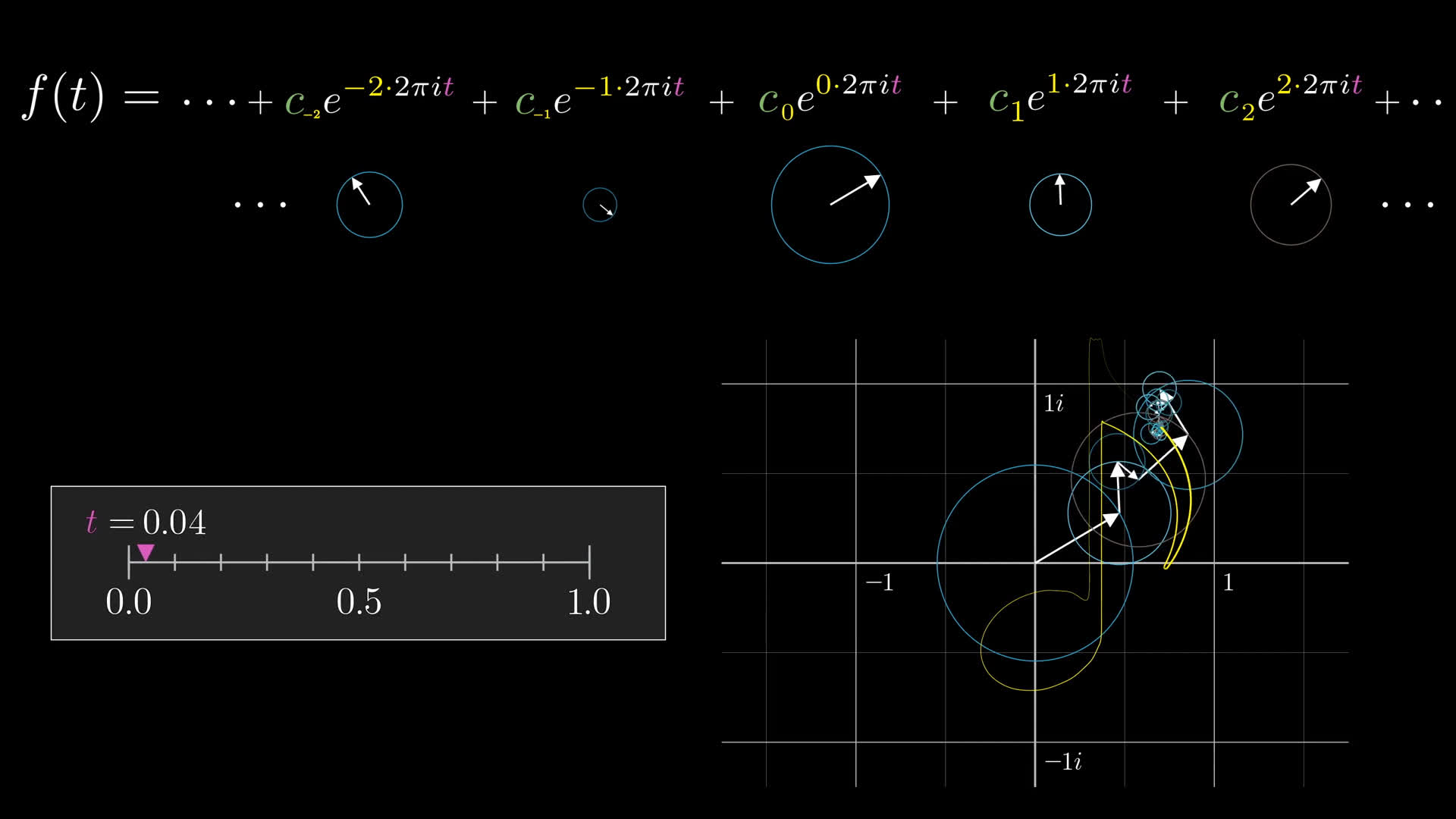
Everyone in our infinite family of rotating vectors has some complex constant being multiplied into it which determines its initial angle and magnitude. Our goal is to express any arbitrary function f(t), say the one below drawing an eighth note, as a sum of terms like this, so we need some way to pick out these constants one-by-one given the data of the function.
The integration trick
The easiest one is the constant term. This term represents a sort of center of mass for the full drawing; if you were to sample a bunch of evenly spaced values for the input t as it ranges from 0 to 1, the average of all the outputs of the function for those samples will be the constant term c_0
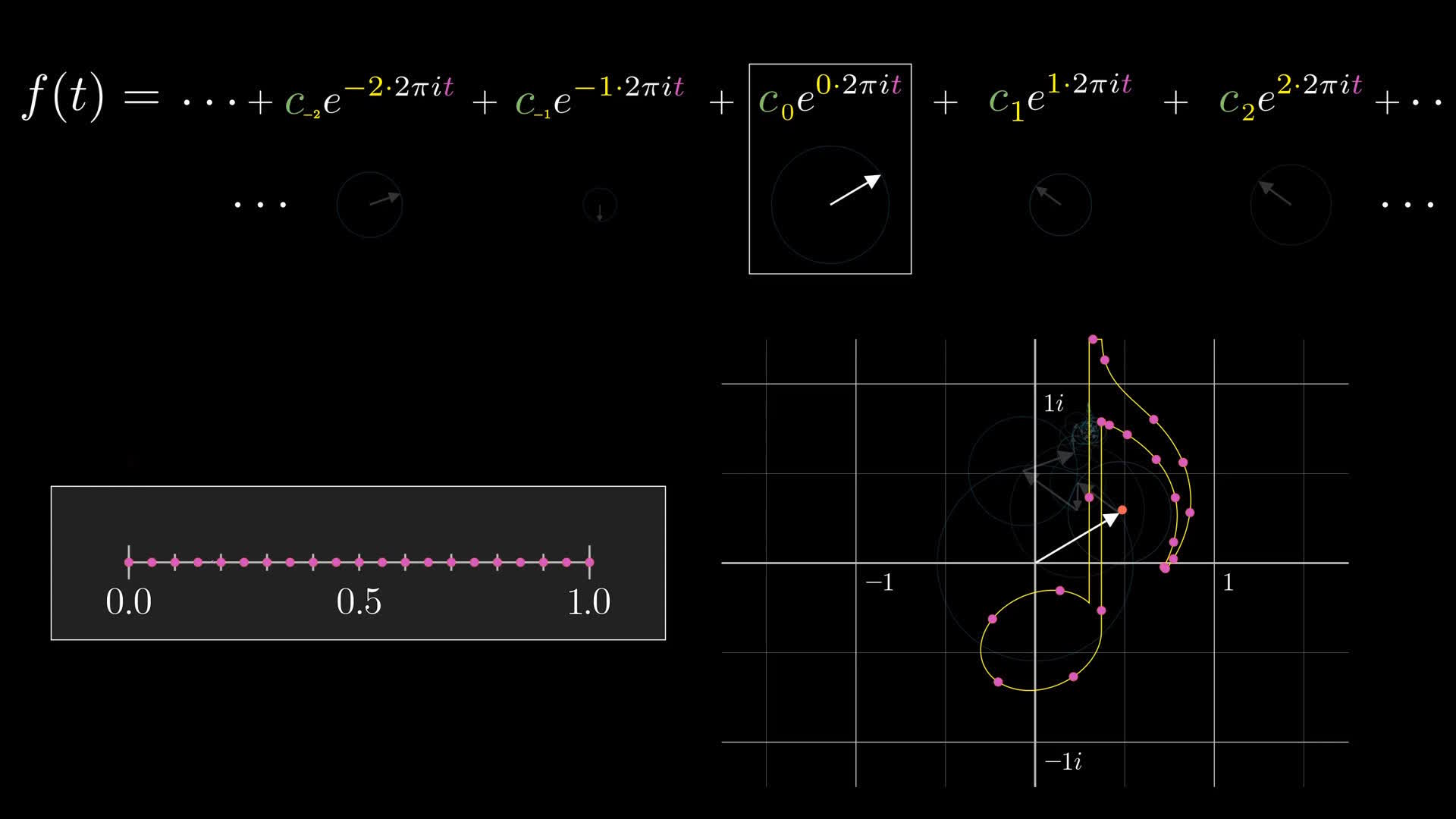
Or more accurately, as you consider finer and finer samples, their average approaches c_0 in the limit.
What I'm describing, finer and finer sums of f(t) for a sample of t from the input range, is an integral of f(t) from 0 to 1.
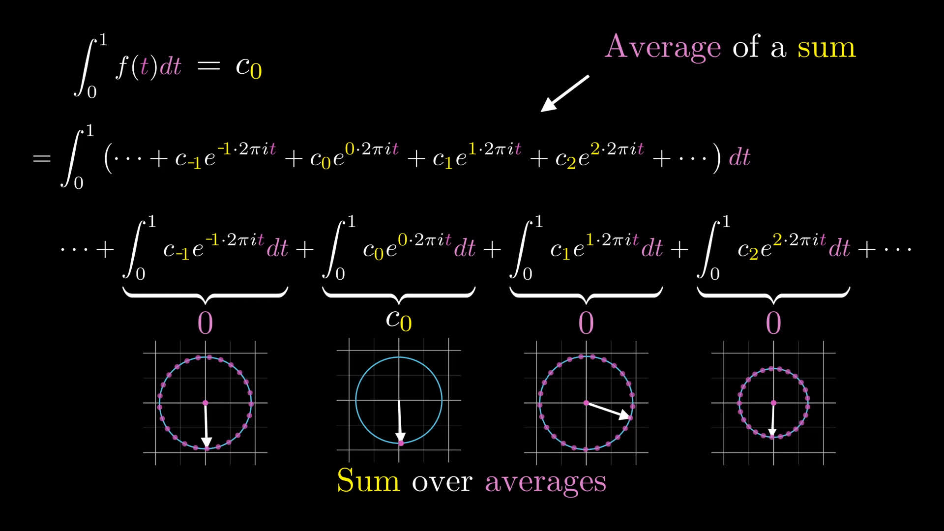
c_0 = \int_{0}^{1} f(t) dtNormally, since the aim is to compute an average, you'd divide this integral by the length of the interval. But that length is 1, so it amounts to the same thing.
c_0 = \frac{1}{1-0} \int_{0}^{1} f(t) dtThere's a very nice way to think about why this integral would pull out c_0. Since we want to think of the function as a sum of these rotating vectors, consider this integral (this continuous average) as being applied to that sum.
\int_{0}^{1} f(t) dt =\int_{0}^{1}\left(\cdots+c_{-1} e^{-1 \cdot 2 \pi i t}+c_{0} e^{0 \cdot 2 \pi i t}+c_{1} e^{1 \cdot 2 \pi i t}+c_{2} e^{2 \cdot 2 \pi i t}+\cdots\right) d tThis average of a sum is the same as a sum over the averages of each part.
=\cdots+\int_{0}^{1} c_{-1} e^{-1 \cdot 2 \pi i t} d t+\int_{0}^{1} c_{0} e^{0 \cdot 2 \pi i t} d t+\int_{0}^{1} c_{1} e^{1 \cdot 2 \pi i t} d t+\int_{0}^{1} c_{2} e^{2 \cdot 2 \pi i t} d t+\cdotsYou can read this move as a shift in perspective. Rather than looking at the sum of all the vectors at each point in time, and taking the average value of the points they trace out, look at the average value for each individual vector as t goes from 0 to 1, and add up all these averages.
It's a subtle shift, but think about what each of those inner integrals being added now means. Each of these rotating vectors makes a whole number of rotations around 0 as t ranges from 0 to 1, so its average value will be 0. The only exception is that constant term; since it stays static and doesn't rotate, its average value is simply whatever number it started on, which is c_0. So doing this average over the whole function kills all the terms except c_0.
Pull out any other term
But now let's say you wanted to compute a different term, like c_2 in front of the vector rotating 2 cycles per second. The trick is to first multiply f(t) by something which makes that vector hold still, the mathematical equivalent of giving a smartphone to an overactive child. Specifically, if you multiply the whole function by e^{-2 \cdot 2 \pi i t}, think about what happens to each term.
Remember, we're assuming you can write f(t) as a sum which looks like this:
f(t) = \left(\cdots
c_{-2}e^{-2 \cdot 2\pi i t} +
c_{-1}e^{-1 \cdot 2\pi i t} +
c_{0}e^{0 \cdot 2\pi i t} +
c_{1}e^{1 \cdot 2\pi i t} +
c_{2}e^{2 \cdot 2\pi i t} +
\cdots\right)In short, multiplying by e^{-2 \cdot 2\pi i t} is a way to make the rotating vectors associated with c_2 e^{2 \cdot 2\pi i t} hold still while all the others move around.
Of course, there's nothing special about 2 here. If we replace it with any other n, you have a formula for any other term c_n.
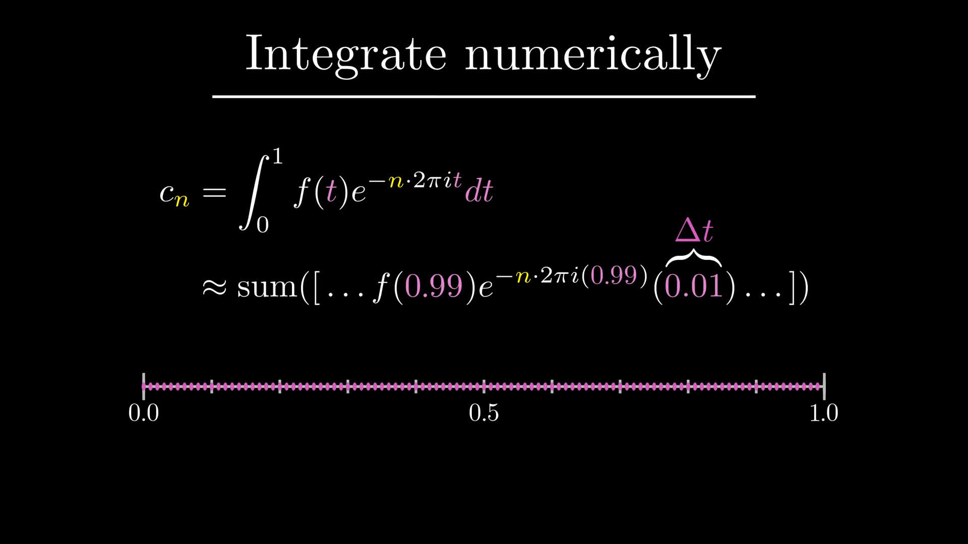
c_n = \int_{0}^{1} f(t) e^{-n \cdot 2 \pi i t} d tAgain, you can read this expression as modifying our function, our 2d drawing, so as to make the n^{\text{th}} little vector hold still, and then performing an average so that all other vectors get canceled out. Isn't that crazy? All the complexity of this decomposition as a sum of many rotations is entirely captured in this expression.
Doing this in practice
To create the animations for this post, that formula is exactly what I'm having the computer evaluate. It treats a path like a complex function, and for a certain range of values for n, it computes this integral to find each coefficient c_n.
For those of you curious about where the data for the path itself comes from, I'm going the easy route having the program read in an svg, which is a file format that defines the image in terms of mathematical curves rather than with pixel values.
Skipping over some details of appropriately massaging the data of those curves, this essentially means the mapping f(t) from a time parameter to points in space comes predefined.
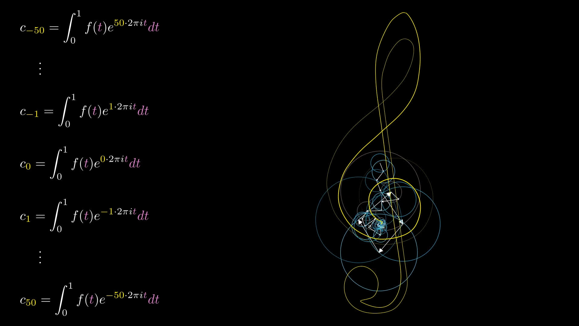
The animation above uses 101 rotating vectors, computing values of n from -50 up to 50. In practice, the integral is computed numerically, essentially meaning it chops up the unit interval into many small pieces of size \Delta t and adds up this value f(t)e^{-n \cdot 2 \pi i t} \Delta t for each one of them. There are fancier methods for more efficient numerical integration, but that gives the basic idea.
After computing these 101 values, each one determines an initial position for the little vectors, and then you set them all rotating, adding them all tip to tail, and the path drawn out by the final tip is some approximation of the original path. As the number of vectors used approaches infinity, it gets more and more accurate.
Relation to step function
To bring this all back down to earth, consider the example we were looking at earlier of a step function, which was useful for modeling the heat dissipation between two rods of different temperatures after coming into contact.
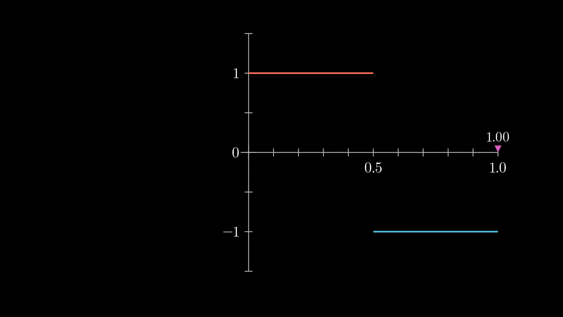
Since it's a real-valued function, a step function is like a boring drawing confined to one-dimension. But this one is an especially dull drawing, since for inputs between 0 and 0.5, the output just stays static at the number 1, and then it discontinuously jumps to -1 for inputs between 0.5 and 1.
What does this mean for the Fourier series approximation? The vector sum stays really close to 1 for the first half of the cycle, then really quickly jumps to -1 for the second half. Remember, each pair of vectors rotating in opposite directions correspond to one of the cosine waves we were looking at earlier.
To find the coefficients, you'd need to compute this integral. For the ambitious reader among you itching to work out some integrals by hand, this is one where you can do the calculus to get an exact answer, rather than just having a computer do it numerically for you. I'll leave it as an exercise to work this out, and to relate it back to the idea of cosine waves by pairing off the vectors rotating in opposite directions.
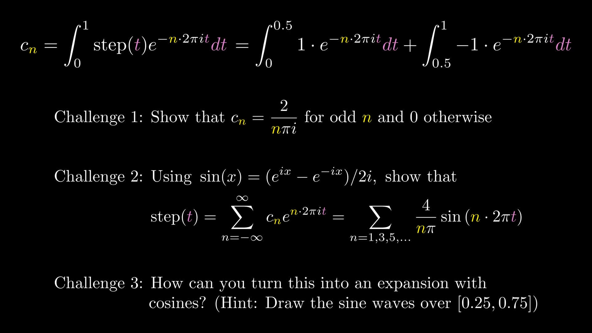
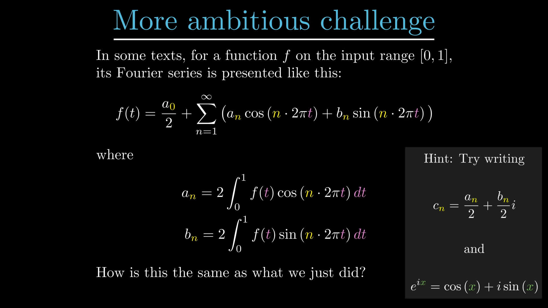
For the even more ambitious, I'll also leave another exercises up on how to relate this more general computation with what you might see in a textbook describing Fourier series only in terms of real-valued functions with sines and cosines.
Conclusion
If you're looking for more Fourier series content, I highly recommend the videos by Mathologer and The Coding Train on the topic, and the blog post by Jezzamoon. Here's an interactive to draw your own path with the corresponding Fourier series.
On the one hand, this concludes our discussion of the heat equation, which was a little window into the study of partial differential equations.
On the other hand, this foray into Fourier series is a first glimpse at a deeper idea. Exponential functions, including their generalization into complex numbers and even matrices, play a very important role for differential equations, especially when it comes to linear equations. What you just saw, breaking down a function as a combination of these exponential functions, comes up again in different shapes and forms.
Thanks
Special thanks to those below for supporting this lesson.