Introduction

After seeing how we think about ordinary differential equations in chapter 1, we turn now to an example of a partial differential equation, the heat equation.

Setup

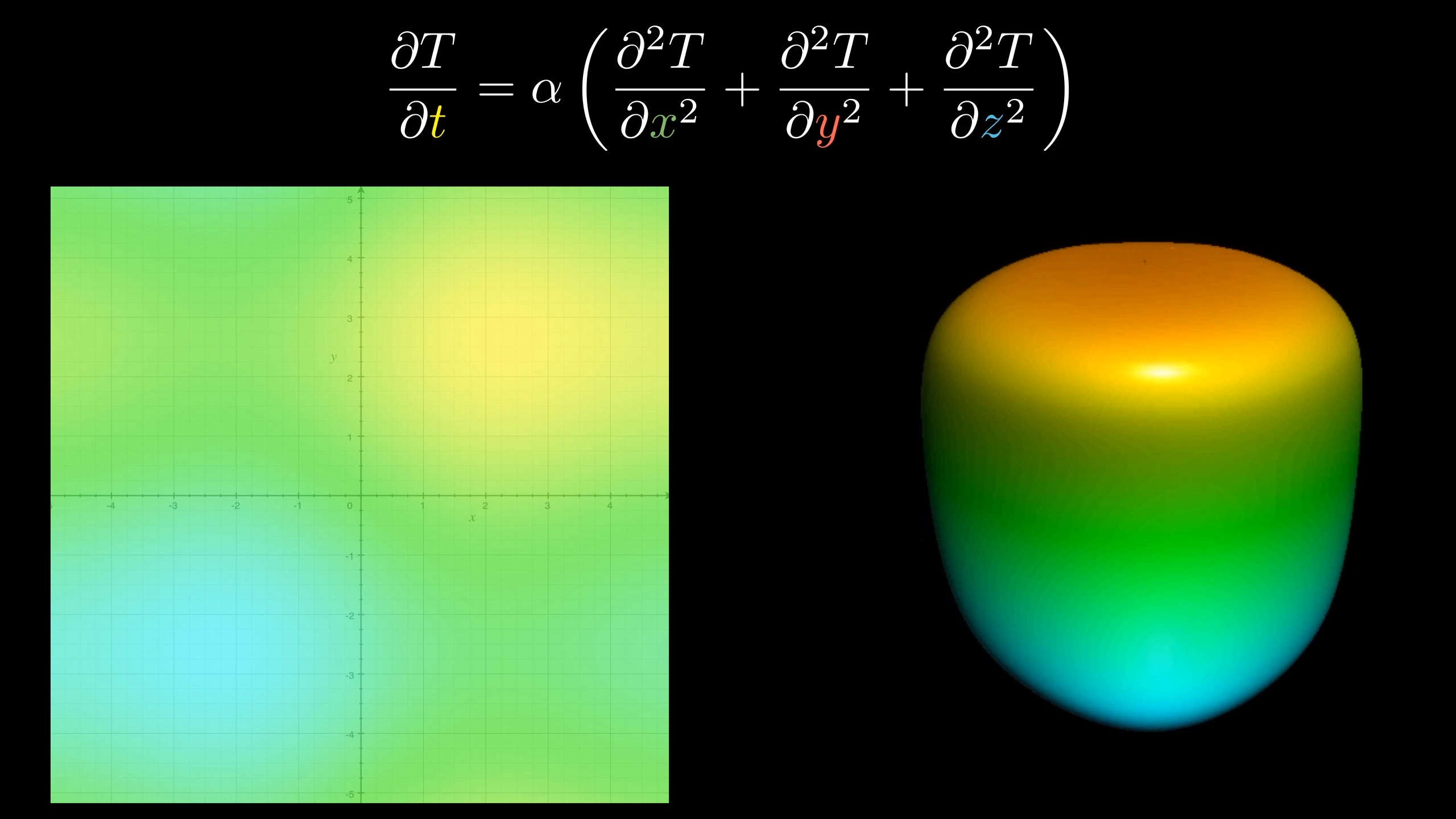
To set things up, imagine you have some object like a piece of metal, and you know how the heat is distributed across it at one moment; what the temperature of every individual point is. You might think of that temperature here as being graphed over the body.

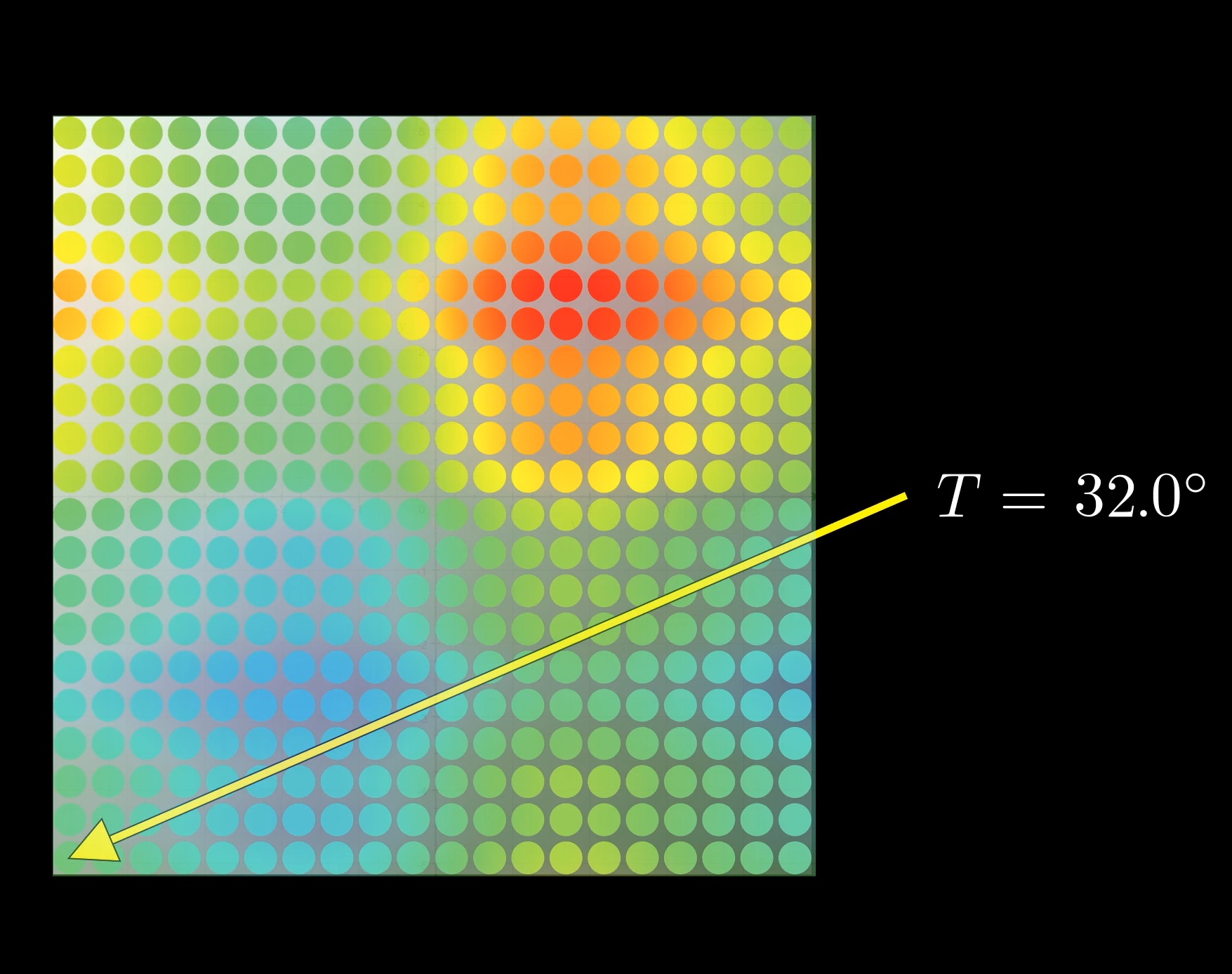
The question is, how will that distribution change over time, as heat flows from the warmer spots to the cooler ones. The image on the left shows the temperature of an example plate with color, with the graph of that temperature being shown on the right, both changing with time.

To take a concrete 1d example, say you have two rods at different temperatures, where that temperature is uniform on each one.

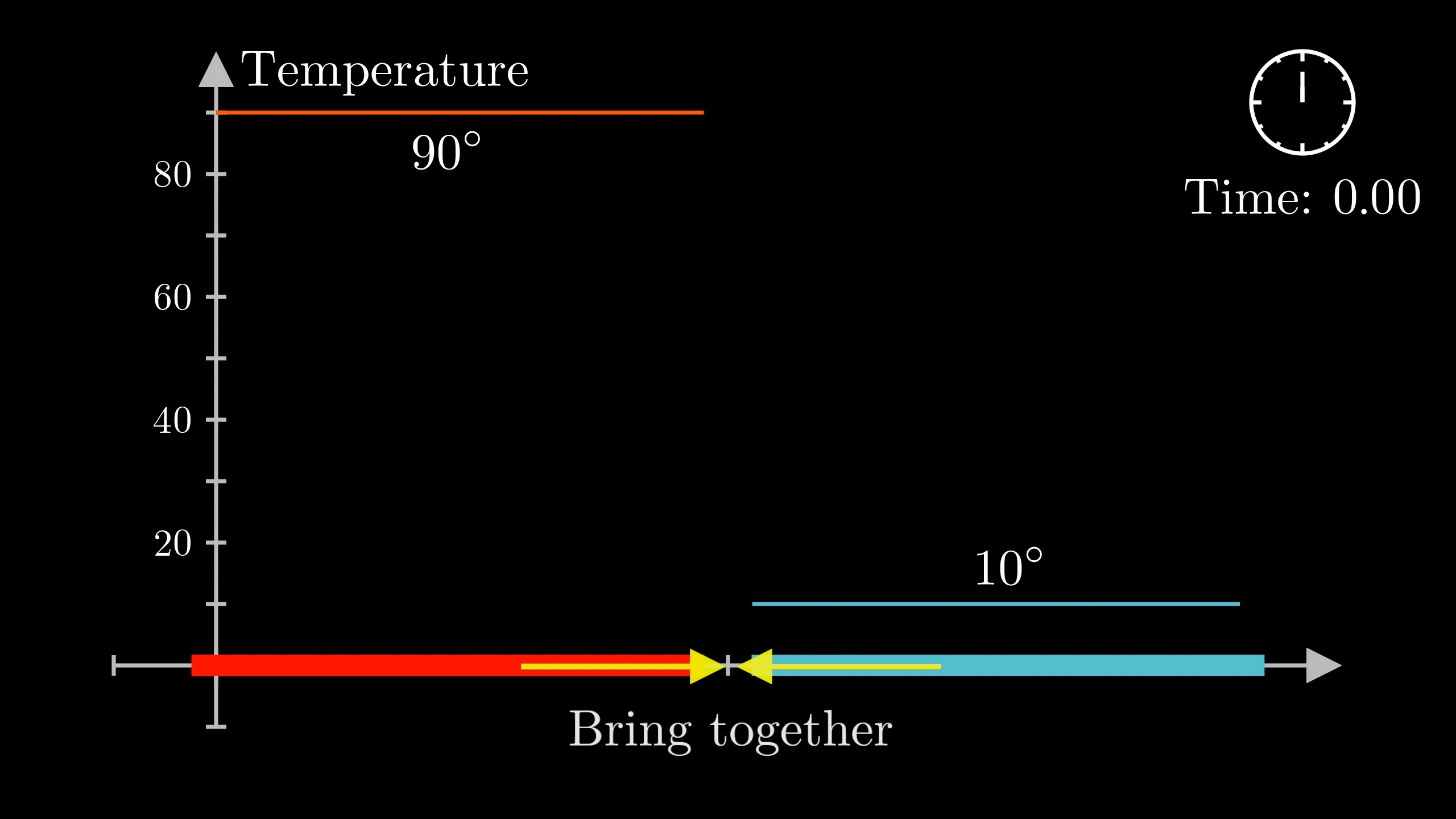
You know that when you bring them into contact, the temperature will tend towards being equal throughout the rod, but how exactly? What will the temperature distribution be at each point in time?

StillAnimation

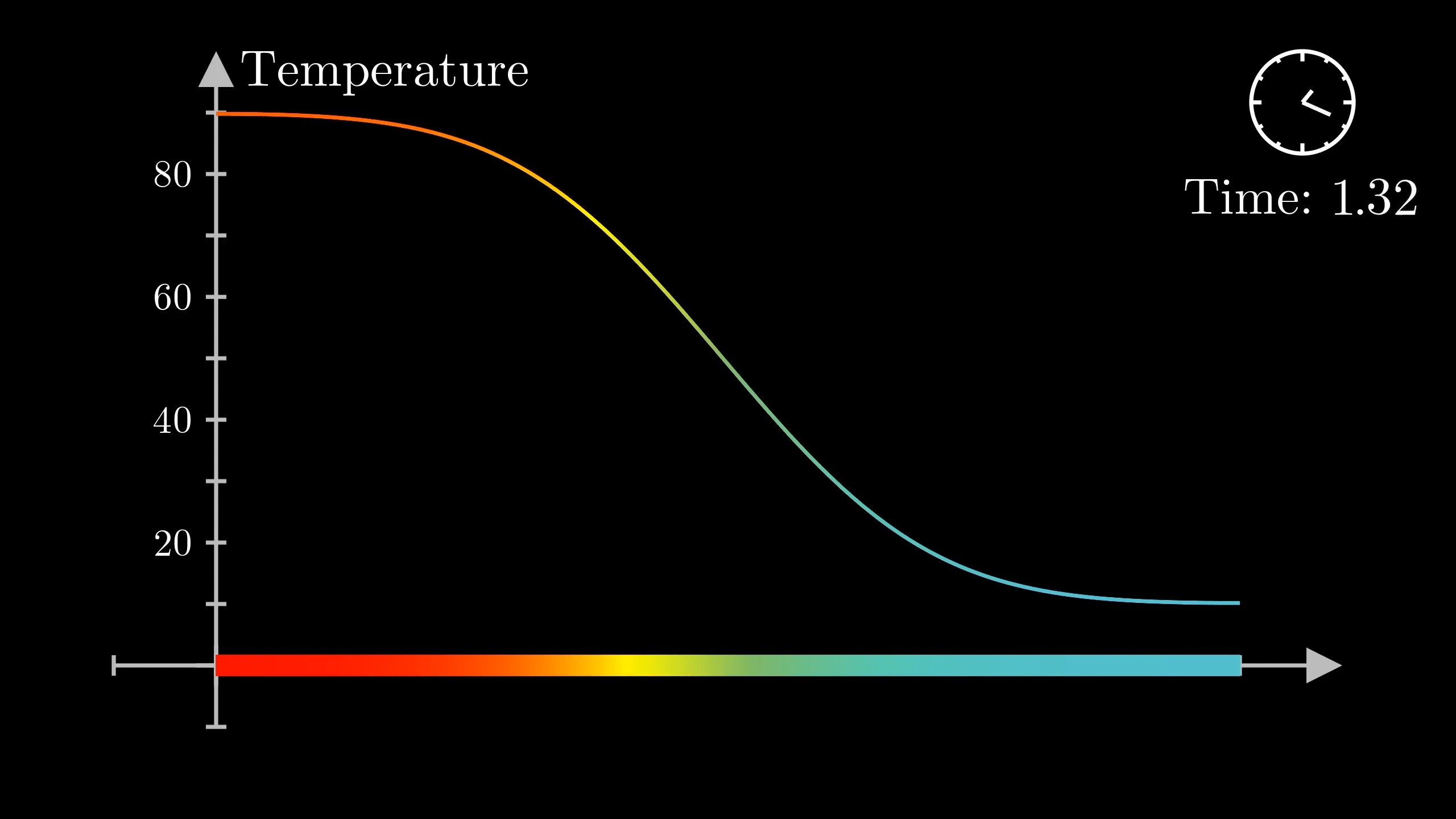
As is typical with differential equations, the idea is that it’s easier to describe how this setup changes from moment to moment than it is to jump to a description of the full evolution. We write this rule of change in the language of derivatives, though as you’ll see we’ll need to expand our vocabulary a bit beyond ordinary derivatives.

What does $\frac{\partial T}{\partial x}$ mean?

Context

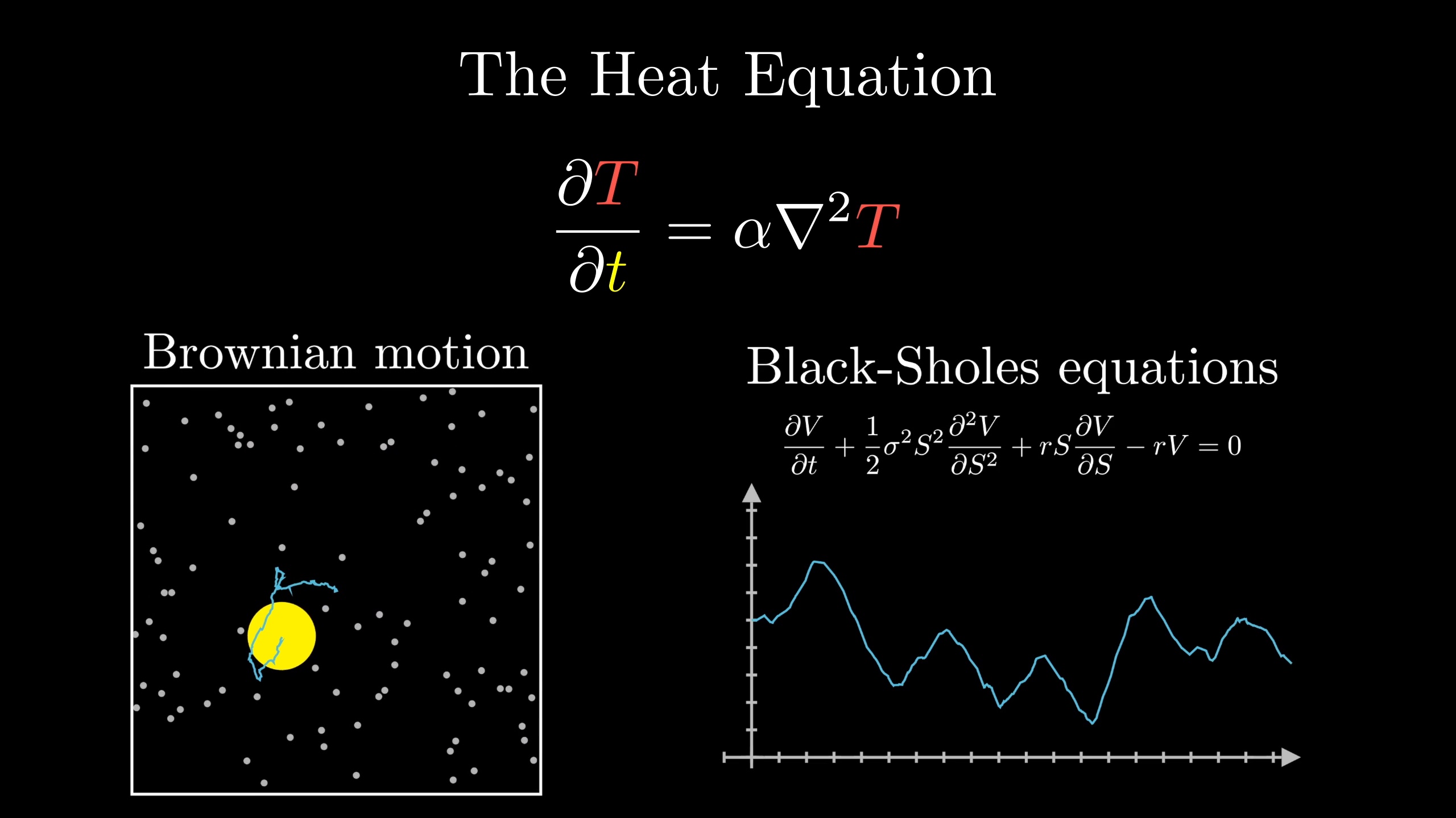
Variations of the heat equation show up in many other parts of math and physics, like brownian motion, the Black-Scholes equations from finance, and all sorts of diffusion, so there are many dividends to be had from a deep understanding of this one setup.

In the last lesson we looked at ways of building understanding while acknowledging the truth that most differential equations are difficult to actually solve.

And indeed, PDEs tend to be even harder than ODEs, largely because they involve modeling infinitely many values changing in concert. But our main character for today is an equation we actually can solve.

If you’ve ever heard of Fourier series, you may be interested to know that this is the physical problem which Fourier was solving when he stumbled across the corner of math now so replete with his name. We’ll dig much more deeply into Fourier series in the next lesson, so be sure to give that one a read after this one.

The heat equation

What does the graph represent?

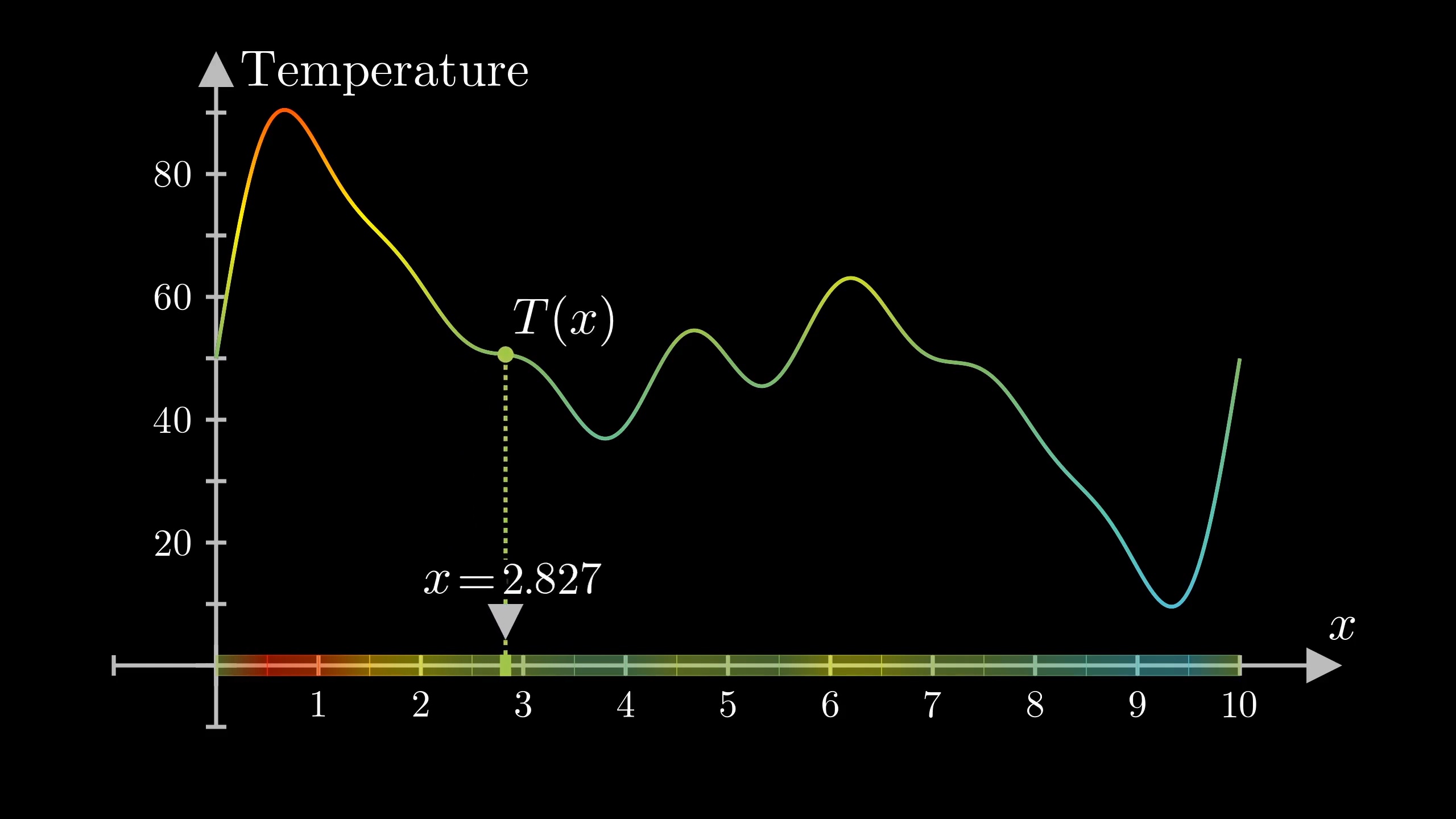
Let's start building up to the heat equation. First, let's be clear on what exactly the function we're analyzing is. We have a rod in one-dimension, and we’re thinking of it as sitting on an $x$-axis, so each point of the rod is labeled with a unique number, $x$. The temperature is some function of that position number, $T(x)$, shown here as a graph above it.

But really, since this value changes over time, we should think of this function as having one more input, $t$ for time. So really, the function we’re analyzing is $T(x, t)$.

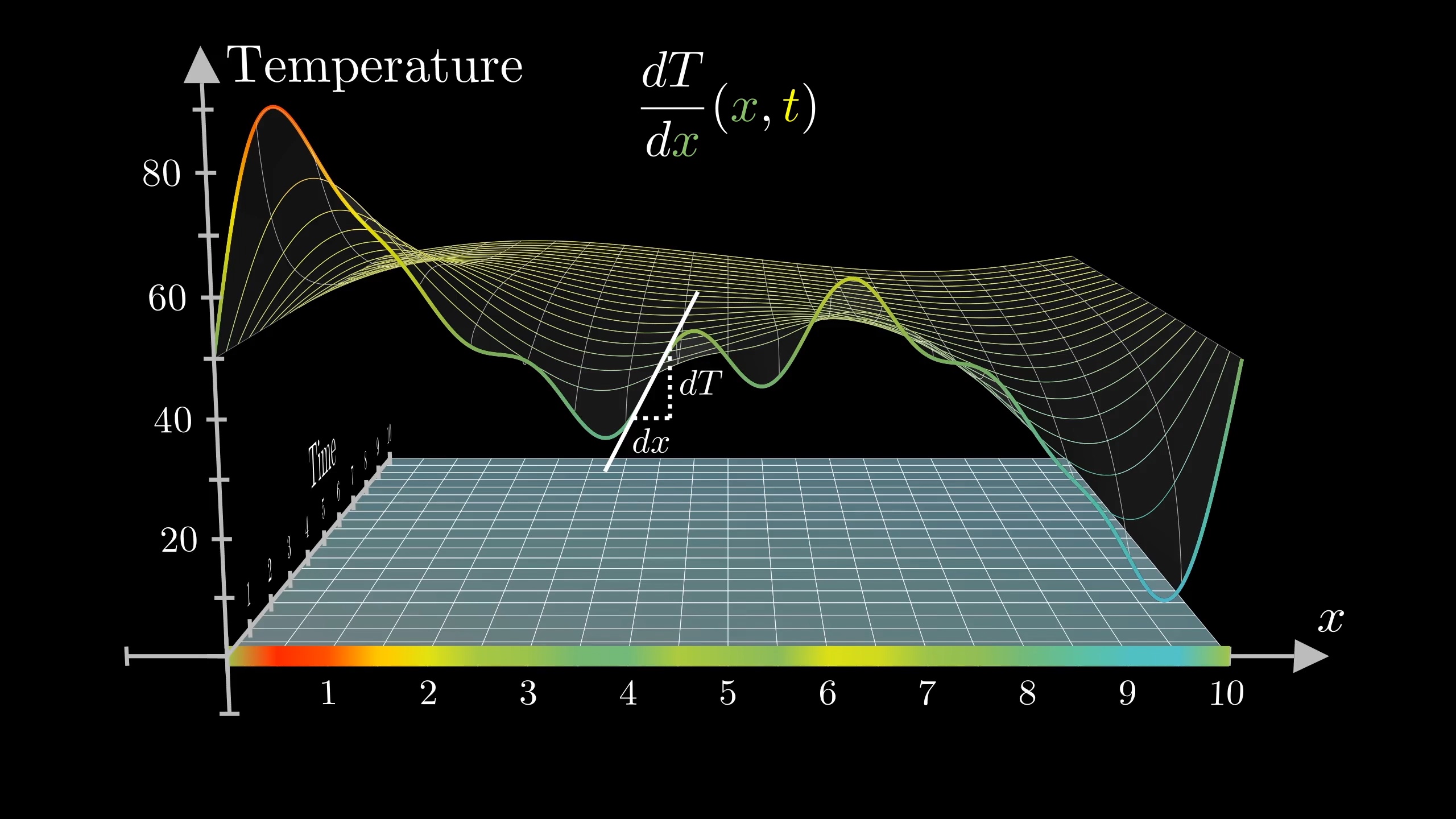
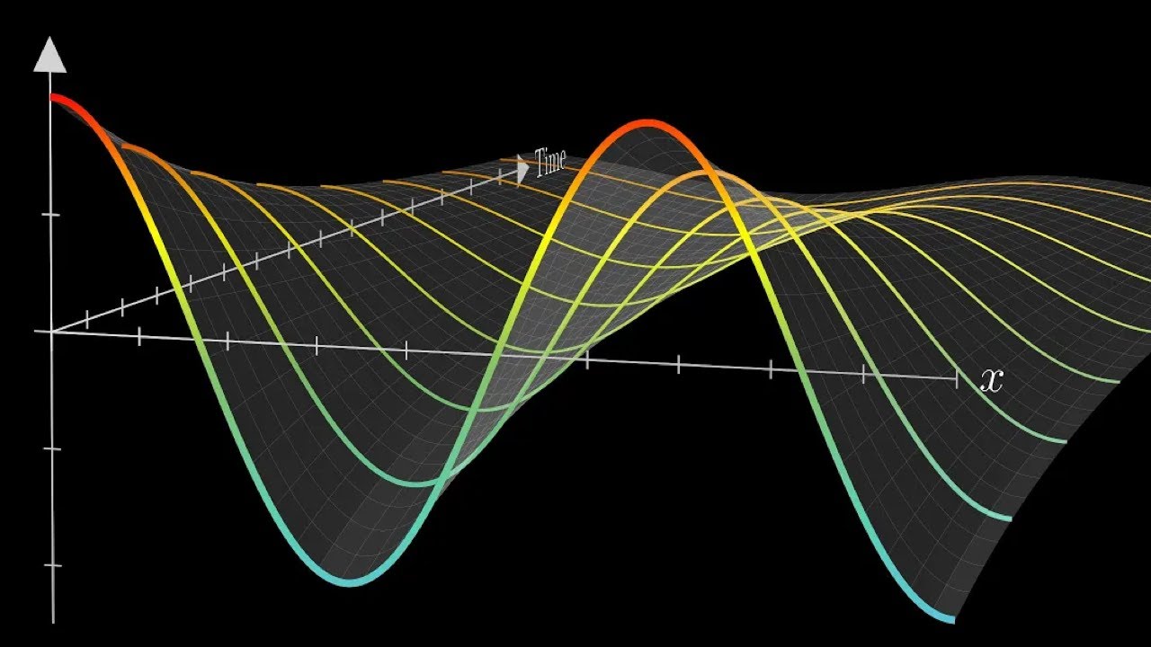
You could, if you wanted, think of the input space as a two-dimensional plane, representing space and time, with the temperature being graphed as a surface above it, each slice across time showing you what the distribution looks like at a given moment.

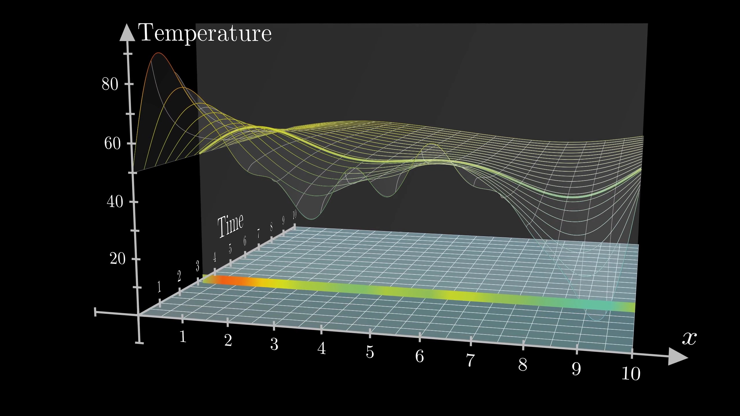
Or you could simply think of the graph of the temperature changing over time. Both are equivalent.

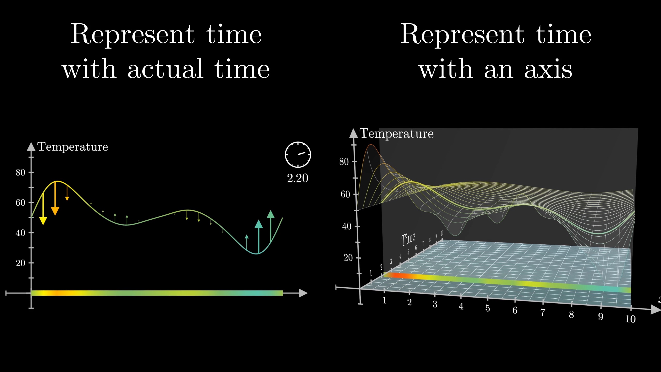
This surface is not to be confused with what I was showing earlier, the temperature graph of a two-dimensional body. Be mindful of whether time is being represented with its own axis, or if it’s being represented with an animation showing literal changes over time.

What are partial derivatives?

In the last chapter, we looked at some systems where just a handful of numbers changed over time, like the angle and angular velocity of a pendulum, describing that change in the language of derivatives. But when we have an entire function changing with time, the mathematical tools become slightly more intricate. Because we’re thinking of this temperature as a function with multiple dimensions to its input space, in this case one for space and one for time, there are multiple different rates of change at play.

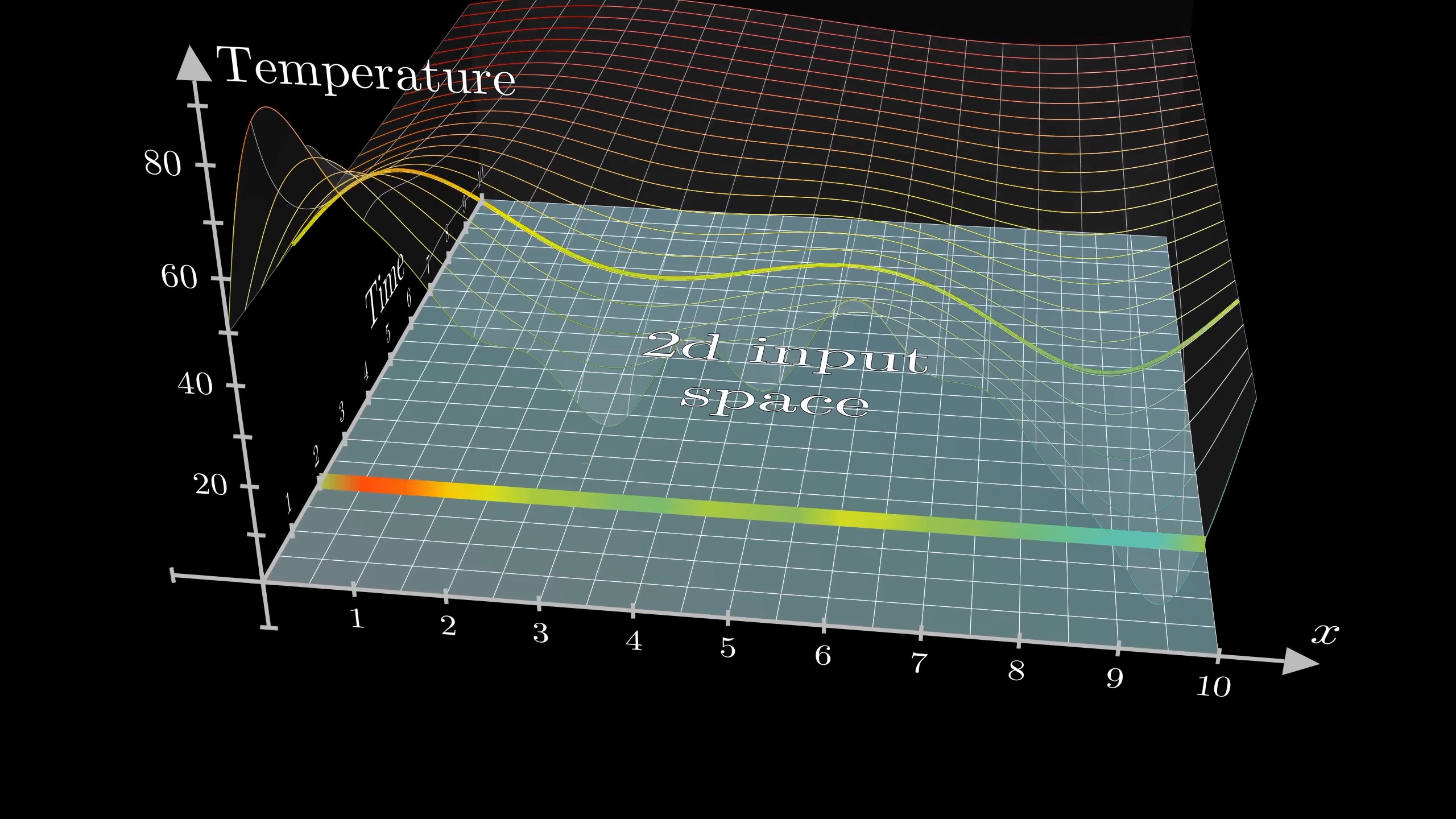
There’s the derivative with respect to $x$; how rapidly the temperature changes as you move along the rod. You might think of this as the slope of our surface when you slice it parallel to the $x$-axis; given a tiny step in the $x$-direction, and the tiny change to temperature caused by it, what’s the ratio?

$\Large\frac{dT}{dx}$

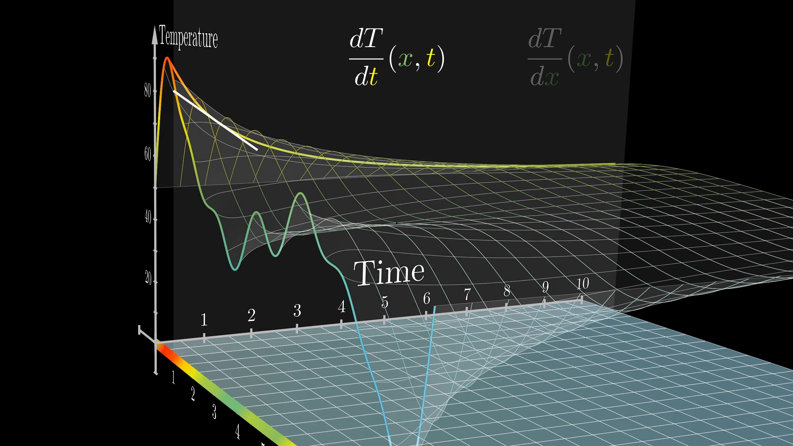
Then there’s the rate of change with time, which you might think of as the slope of this surface when we slice it in a direction parallel to the time axis.

$\Large\frac{dT}{dt}$

Each one of these derivatives only tells part of the story of how the temperature function changes, so we call them “partial derivatives”. To emphasize this point, the notation changes a little, replacing the letter $d$ with $\partial$, sometimes called “del”. ¹

To reiterate a point I made in the calculus series, I do think it's healthy to initially read derivatives like this as a literal ratio between a small change to a function's output, and the small change to the input that caused it. Just keep in mind that what this notation is meant to convey is the limit of that ratio for smaller and smaller nudges to the input, rather than for some specific finitely small nudge. This goes for partial derivatives just as it does for ordinary derivatives, and I believe can make partial derivatives easier to reason about.

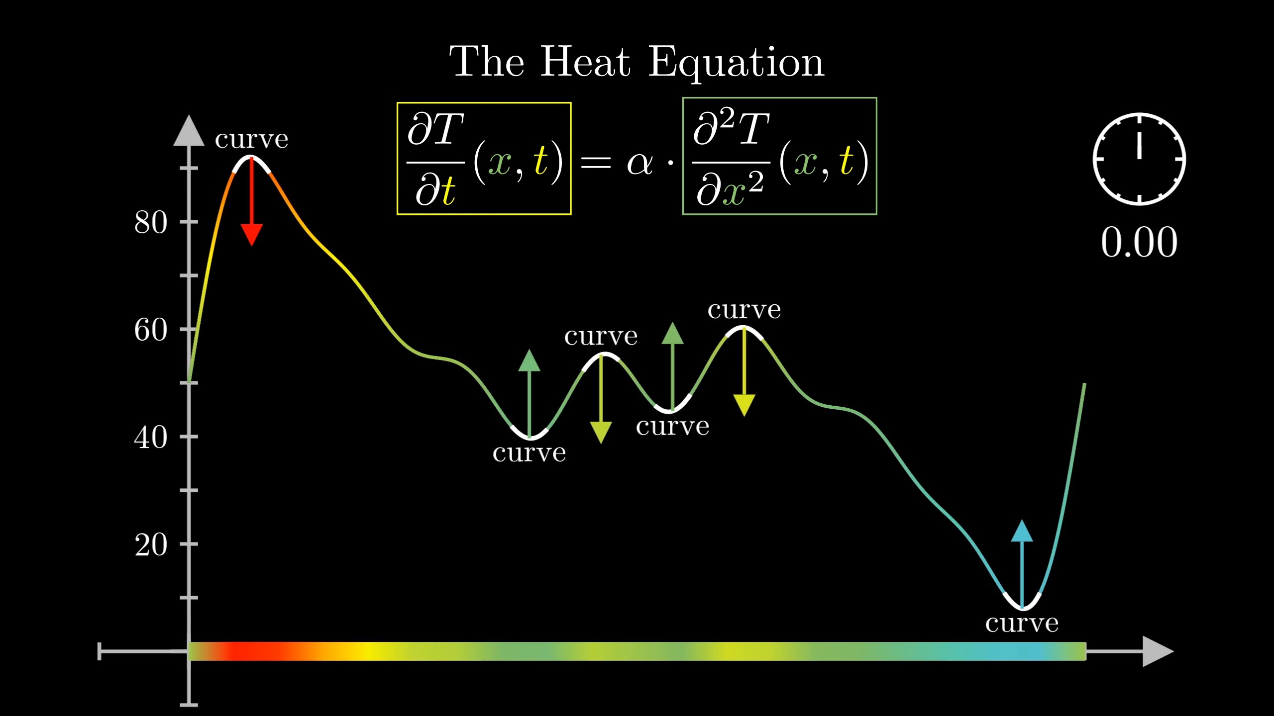
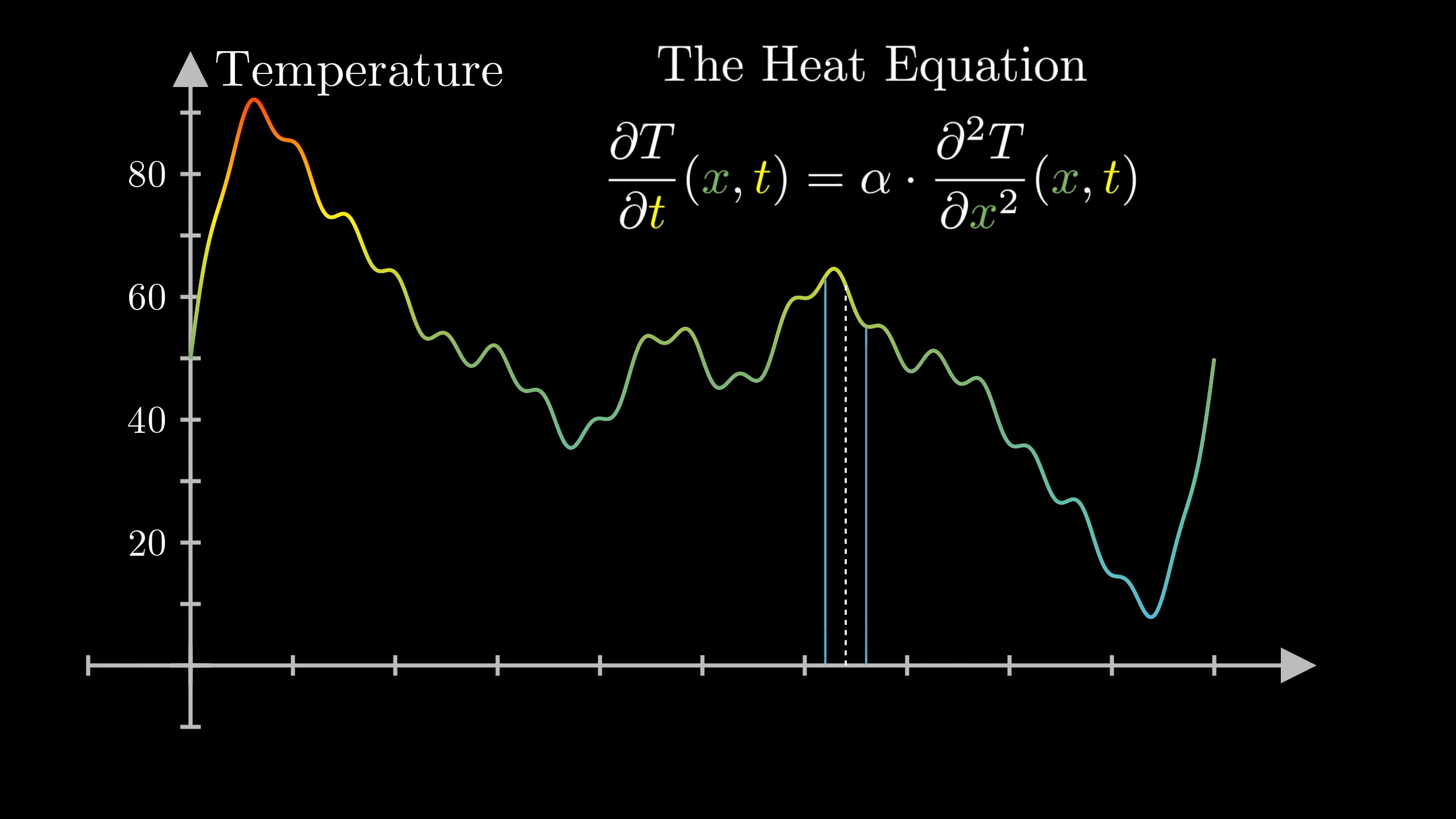
The heat equation is written in the language of partial derivatives.

It states that the way the temperature changes with respect to time depends on its second derivative with respect to space. At a high level, the intuition is that at points where the temperature distribution curves, it tends to change in the direction of that curvature.

Since a rule like this is written with partial derivatives, we call it a partial differential equation. This has the funny result that to an outsider, the name sounds like a tamer version of ordinary differential equations, when to the contrary partial differential equations tend to tell a much richer story than ODEs.

The general heat equation applies to bodies in any number of dimensions, which would mean more inputs to our temperature function, but it’ll be easiest for us to stay focused on the one-dimensional case of a rod.

As it is, graphing this in a way which gives time its own axis already pushes the visuals into three-dimensions.

The discrete case

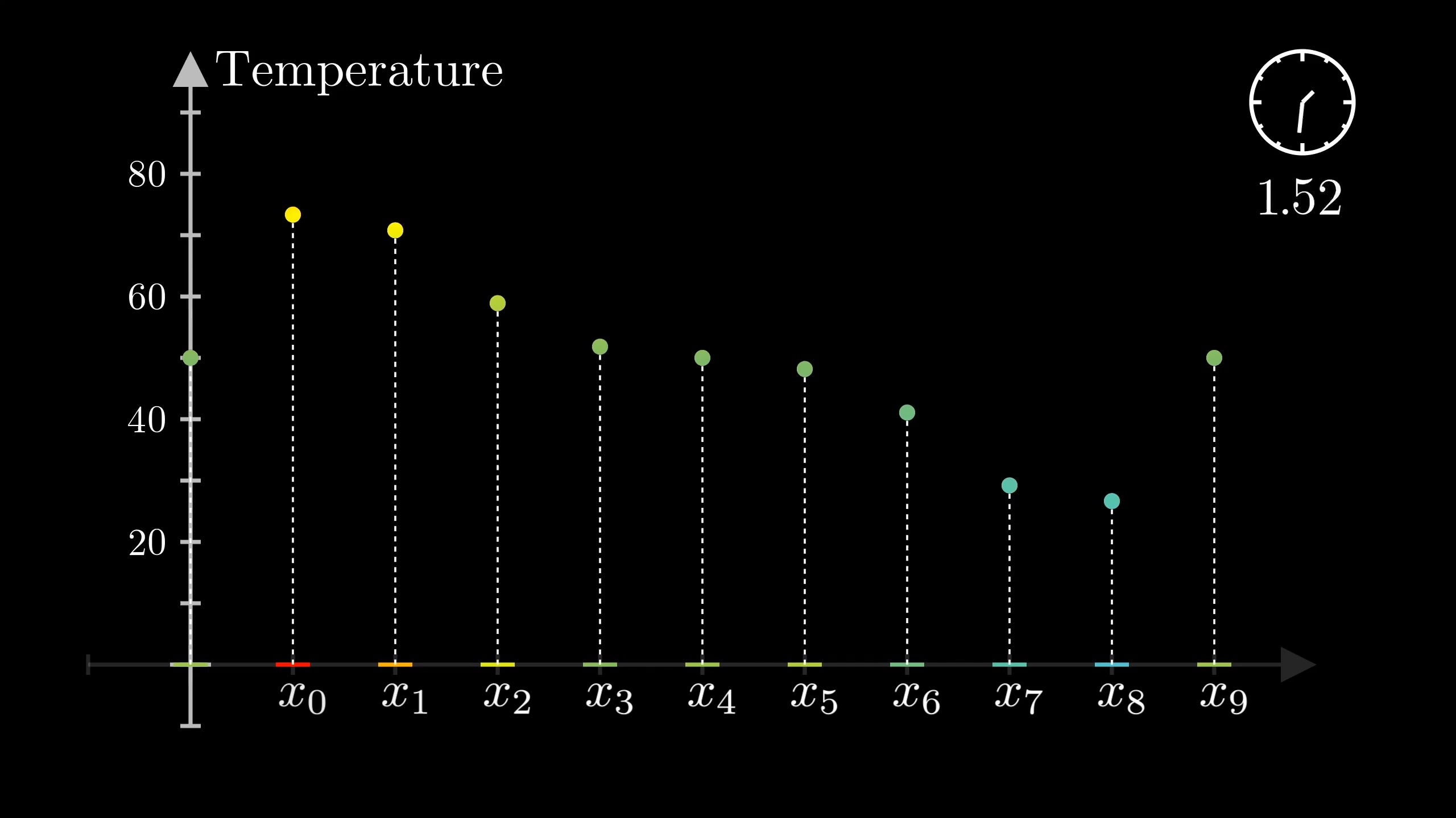
But where does an equation like this come from? How could you have thought this up yourself? Well, for that, let’s simplify things by describing a discrete version of this setup, where you have only finitely many points x in a row. This is sort of like working in a pixelated universe, where instead of having a continuum of temperatures, we have a finite set of separate values.

If the two neighbours are cooler on average, it will cool down.

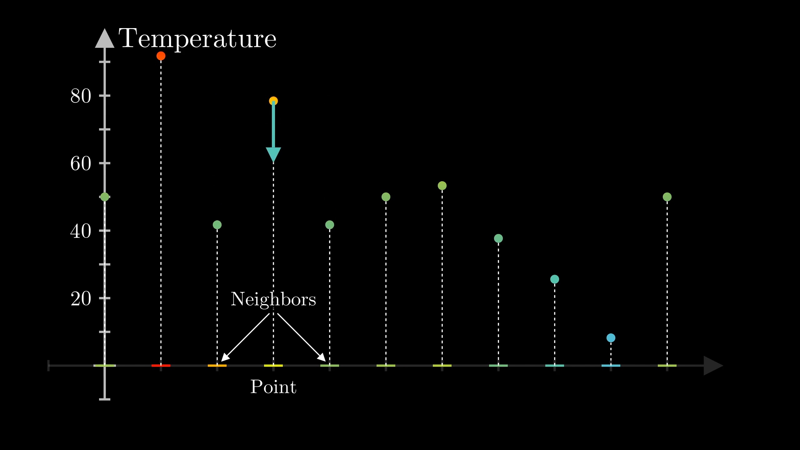
Focus on three neighboring points, $x_1, x_2$ and $x_3$, with corresponding temperatures $T_1, T_2,$ and $T_3$. What we want to compare is the average of $T_1$ and $T_3$ with the value of $T_2$.

When this difference is greater than $0$, $T_2$ will tend to heat up. And the bigger the difference, the faster it heats up.

Likewise, if it’s negative, $T_2$ will cool down, ak a rate proportional to the difference.

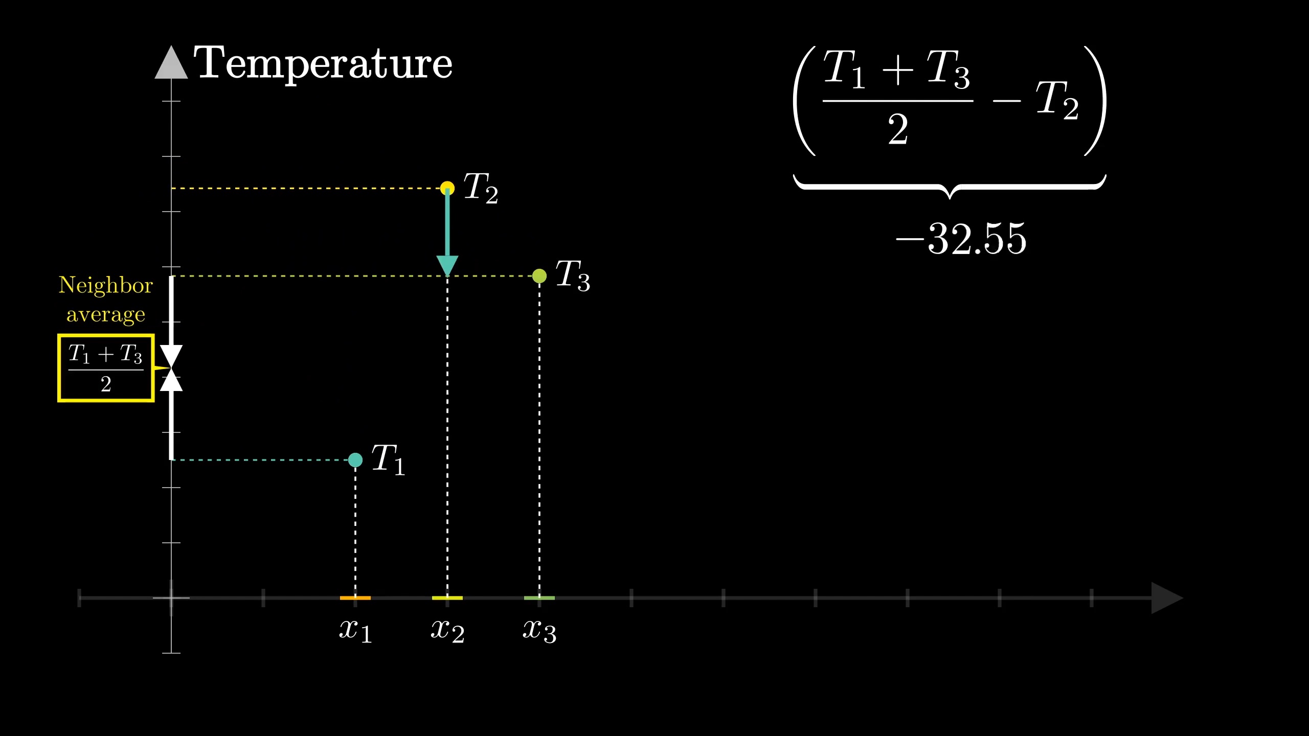
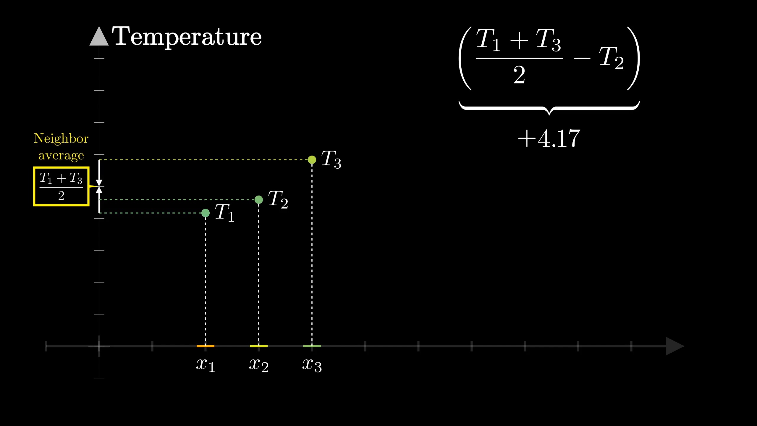
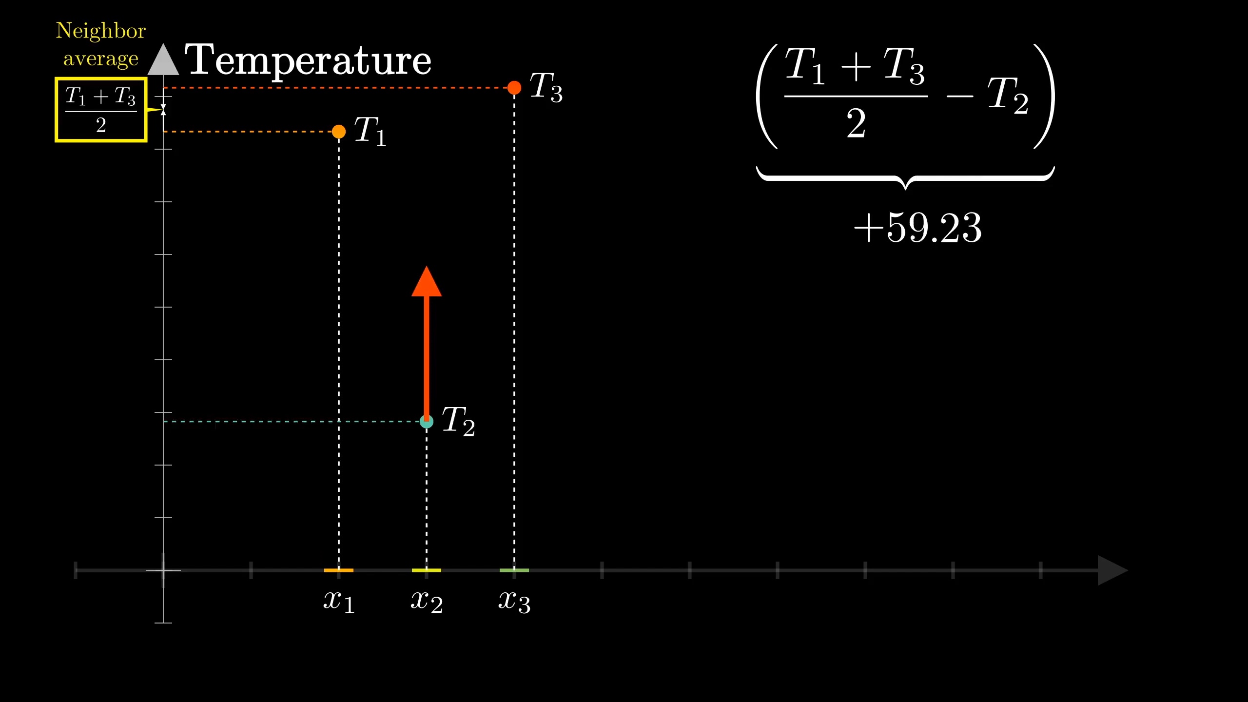
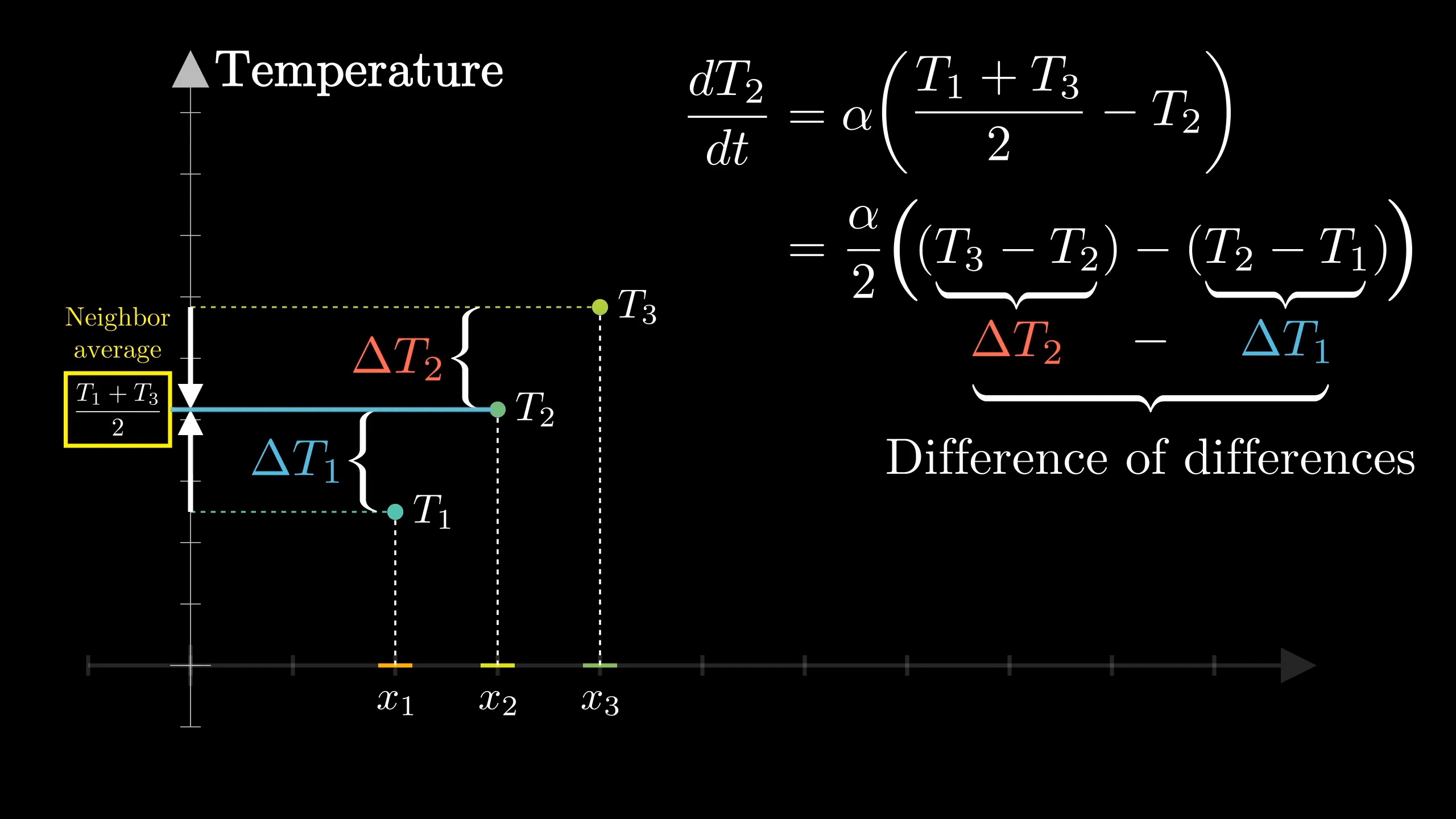
More formally, the derivative of $T_2$, with respect to time, is proportional to this difference between the average value of its neighbors and its own value. Alpha, here, is simply a proportionality constant.

To write this in a way that will ultimately explain the second derivative in the heat equation, let me rearrange this right hand side in terms of the difference between $T_3$ and $T_2$ and the difference between $T_2$ and $T_1$. ²

Like I said, the reason to rewrite it is that it takes a step closer to the language of derivatives. Let’s write these as $\Delta T_1$ and $\Delta T_2$.

It’s the same number, but we’re adding a new perspective. Instead of comparing the average of the neighbors to $T_2$, we’re thinking of the difference of the differences. Here, take a moment to gut-check that this makes sense.

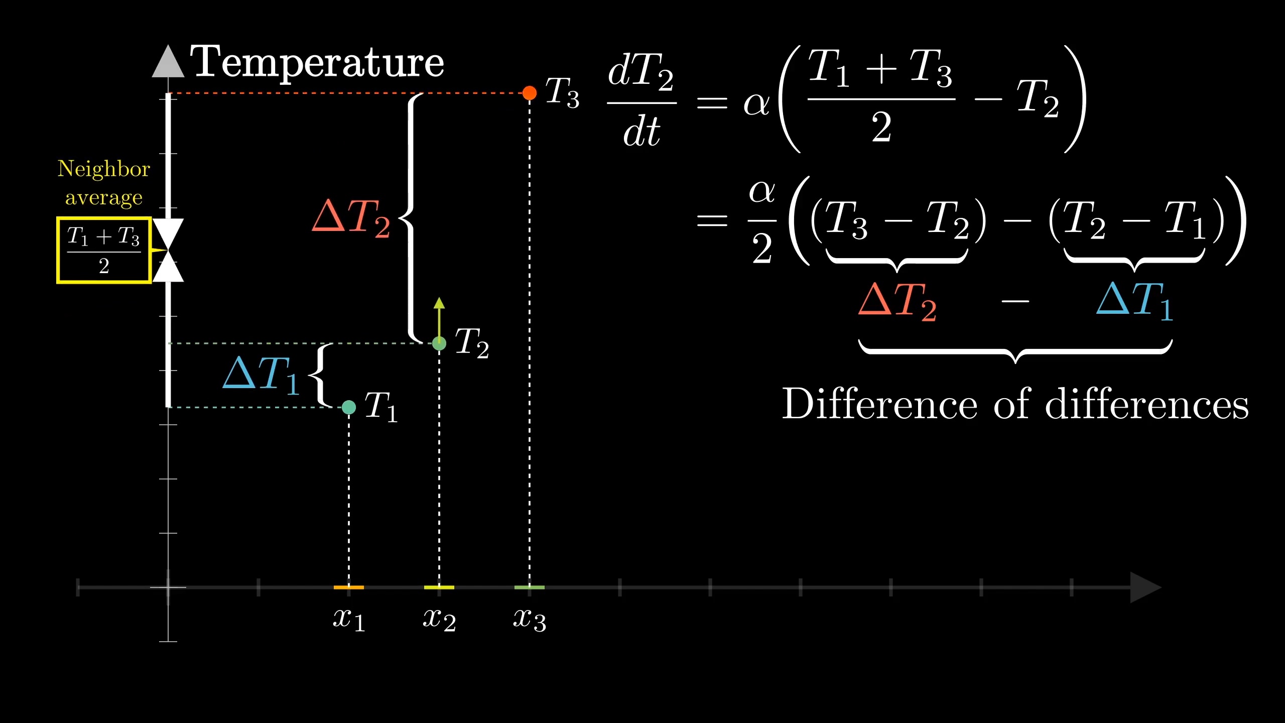
If those two differences are the same, then the average of $T_1$ and $T_3$ is the same as $T_2$, so $T_2$ will not tend to change.

If $\Delta T_2 > \Delta T_1$, meaning the difference of the differences is positive, notice how the average of $T_1$ and $T_3$ is bigger than $T_2$, so $T_2$ tends to increase.

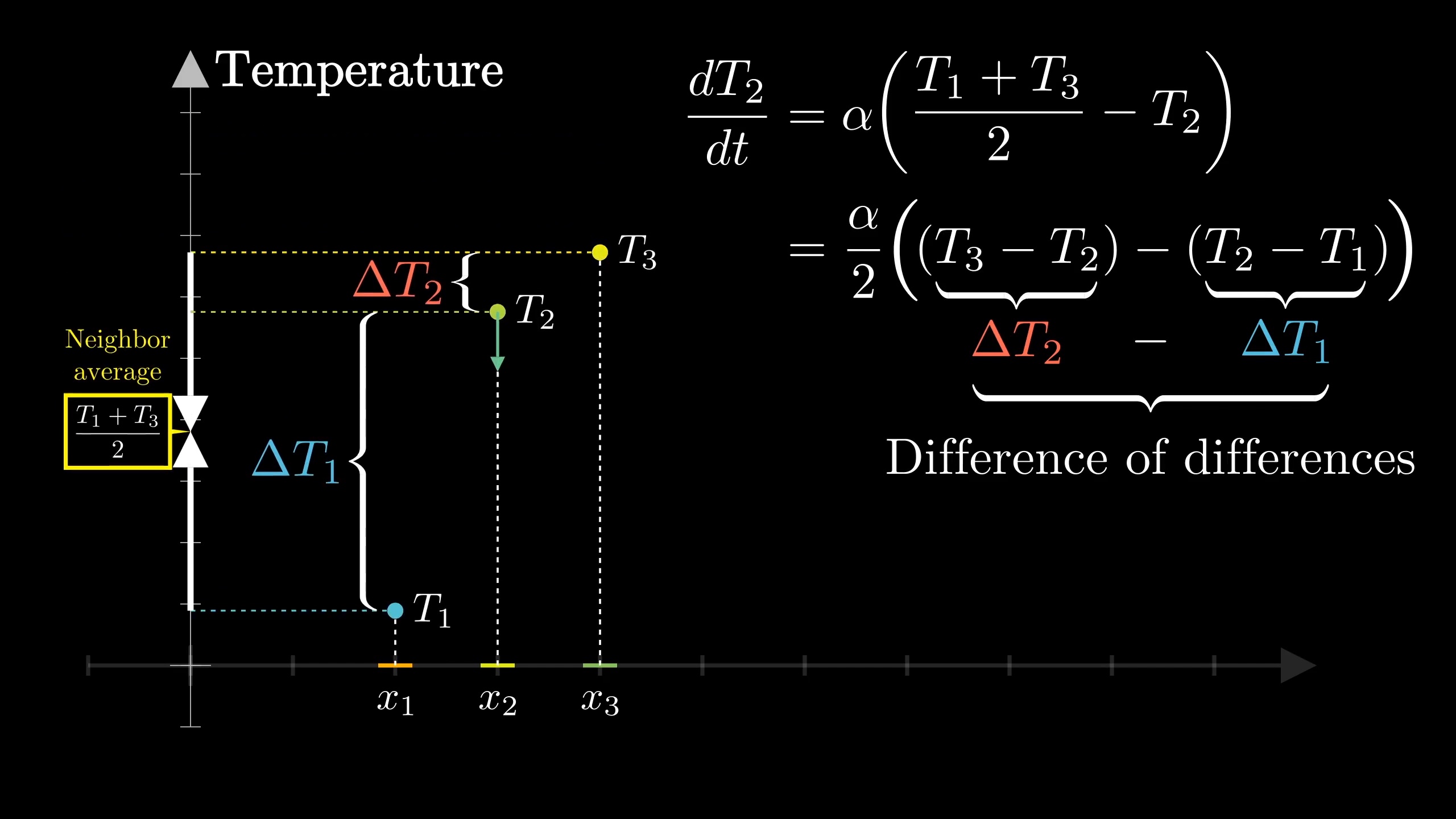
Likewise, if the difference of the differences is negative, meaning $\Delta T_2 < \Delta T_1$, it corresponds to the average of these neighbors being less than $T_2$, and so $T_2$ decreases.

If we wanted to be compact, we could write $\Delta T_2-\Delta T_1$ as $\Delta \Delta T_1$ This is known in the lingo as a “second difference”. If it feels a little weird to think about, keep in mind that it’s essentially a compact way of writing this idea of how much $T_2$ differs from the average of its neighbors, just with an extra factor of $\frac{1}{2}$ is all. That factor doesn’t really matter, because either way we’re writing our equation in terms of some proportionality constant.

The upshot is that the rate of change for the temperature of a point is proportional to the second difference around it.

Transitioning to the continuous case

As we go from this finite context to the infinite continuous case, the analog of a second difference is the second derivative.

Instead of looking at the difference between temperature values at points some fixed distance apart, you consider what happens as you shrink this size of that step towards $0$. And in calculus, instead of asking about absolute differences, which would approach $0$, you think in terms of the rate of change, in this case what’s the rate of change in temperature per unit distance. Remember, there are two separate rates of change at play: How does the temperature change as time progresses, and how does the temperature change as you move along the rod.

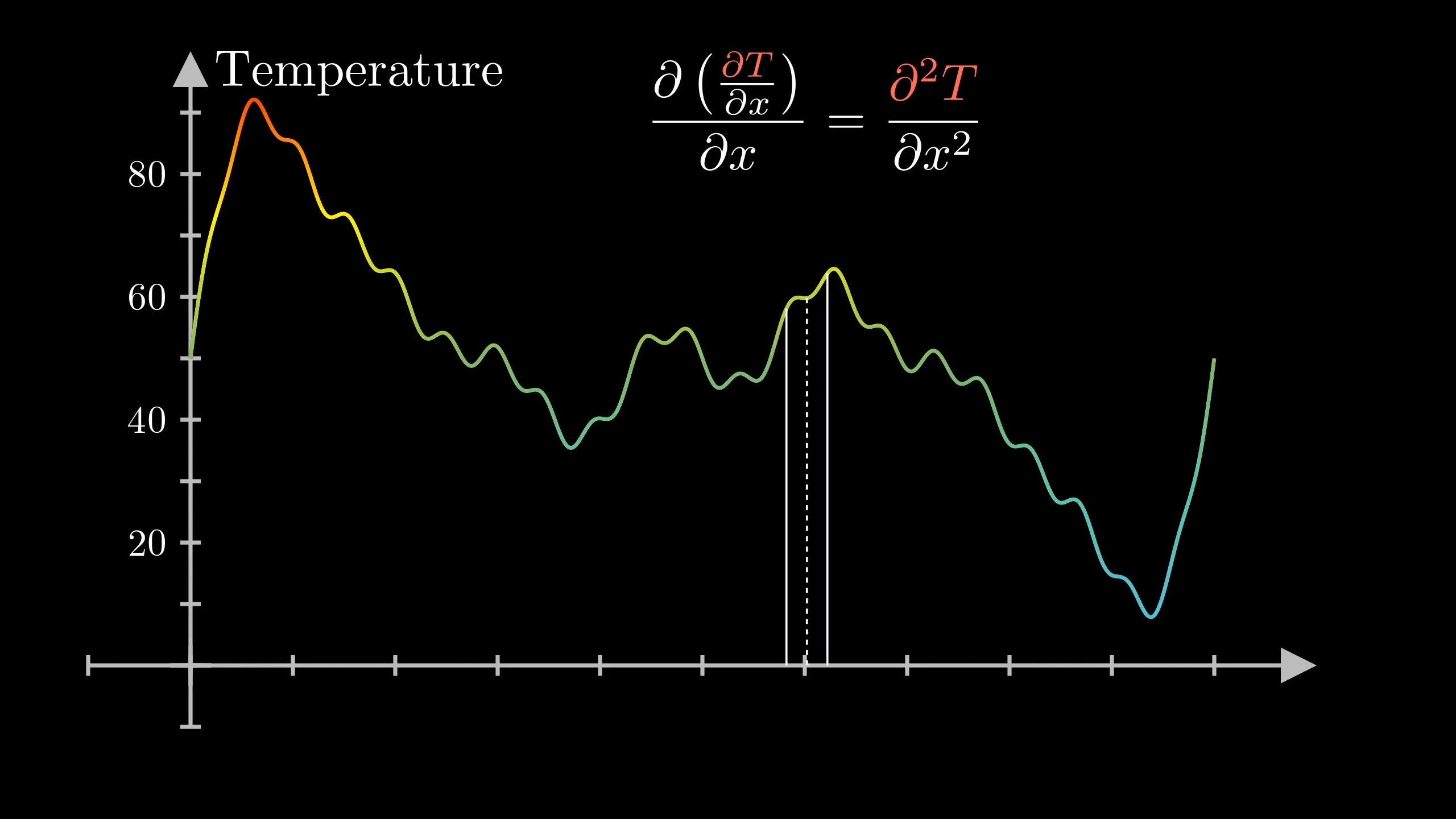
The core intuition remains the same as what we just looked at for the discrete case: To know how a point differs from its neighbors, look not just at how the function changes from one point to the next, but at how that rate of change changes.

This is written as $\frac{\partial^2 T}{\partial x^2}$, the second partial derivative of our function with respect to $x$.

Tuck that away as a meaningful intuition for problems well beyond the heat equation: Second derivatives give a measure of how a value compares to the average of its neighbors.

Hopefully that gives some satisfying added color to this equation. It’s pretty intuitive when reading it as saying curved points tend to flatten out, but I think there’s something even more satisfying seeing a partial differential equation arise, almost mechanistically, from thinking of each point as tending towards the average of its neighbors.

PDEs vs ODEs

Take a moment to compare what this feels like to the case of ordinary differential equations. For example, let's say we have multiple bodies in space, tugging on each other with gravity.

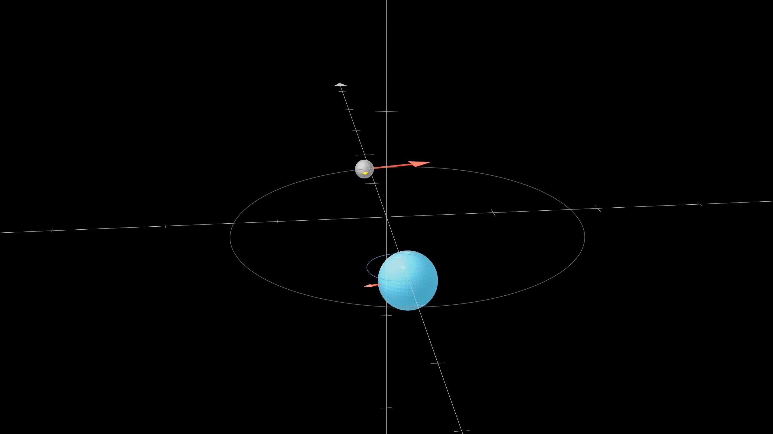
We have a handful of changing numbers: The coordinates for the position and velocity of each body. The rate of change for any one of these values depends on the values of the other numbers, which we write down as a system of equations. On the left, we have the derivatives of these values with respect to time, and the right is some combination of all these values.

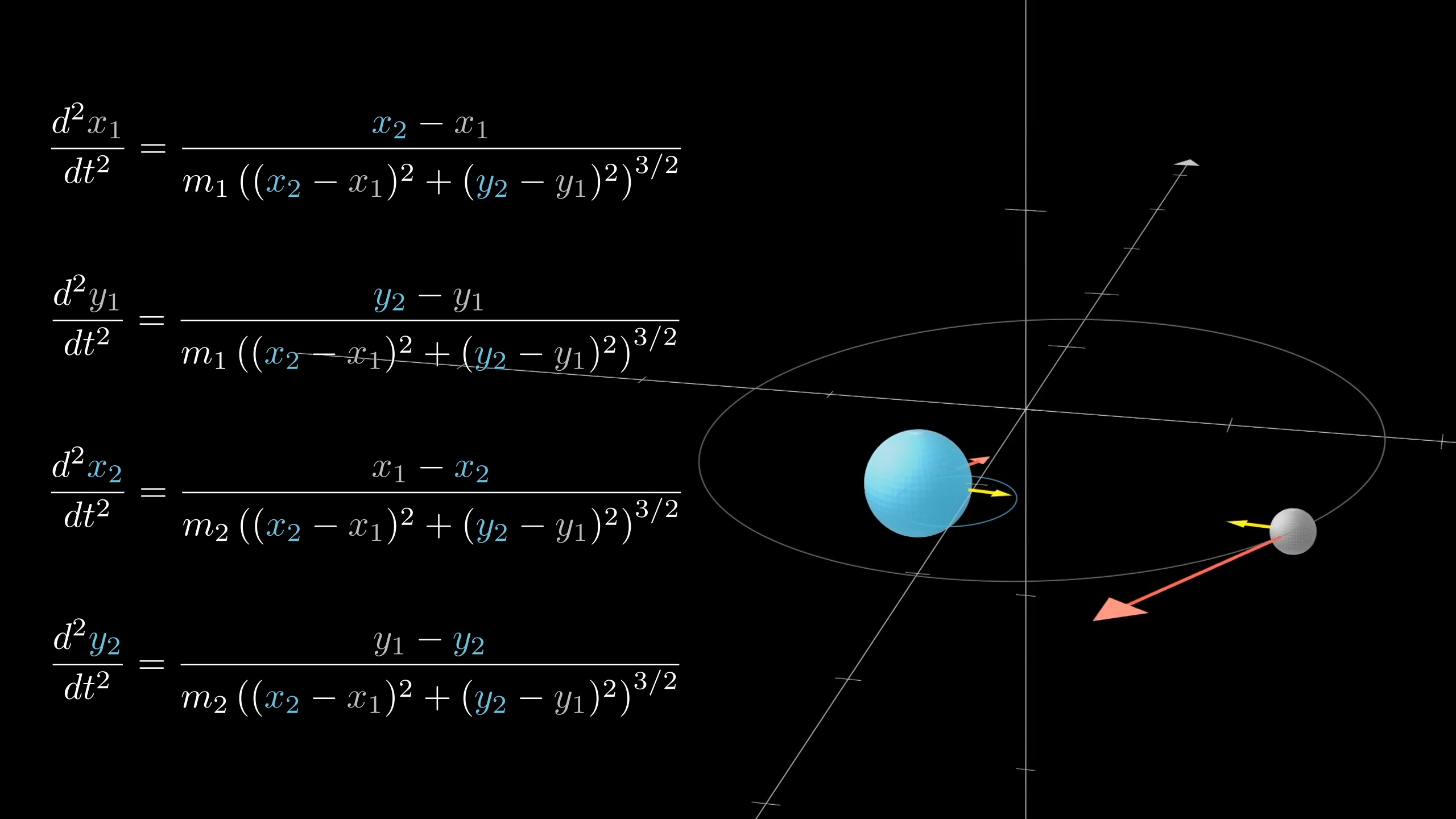
In our partial differential equation, we have infinitely many values from a continuum, all changing. And again, the way any one of these values changes depends on the other values. But helpfully, each one only depends on its immediate neighbors, in some limiting sense of the word neighbor.

So here, the relation on the right-hand side is not some sum or product of the other numbers, it’s also a kind of derivative, just a derivative with respect to space instead of time. In a sense, this one partial differential equation is like a system of infinitely many equations, one for each point on the rod.

Higher dimensions

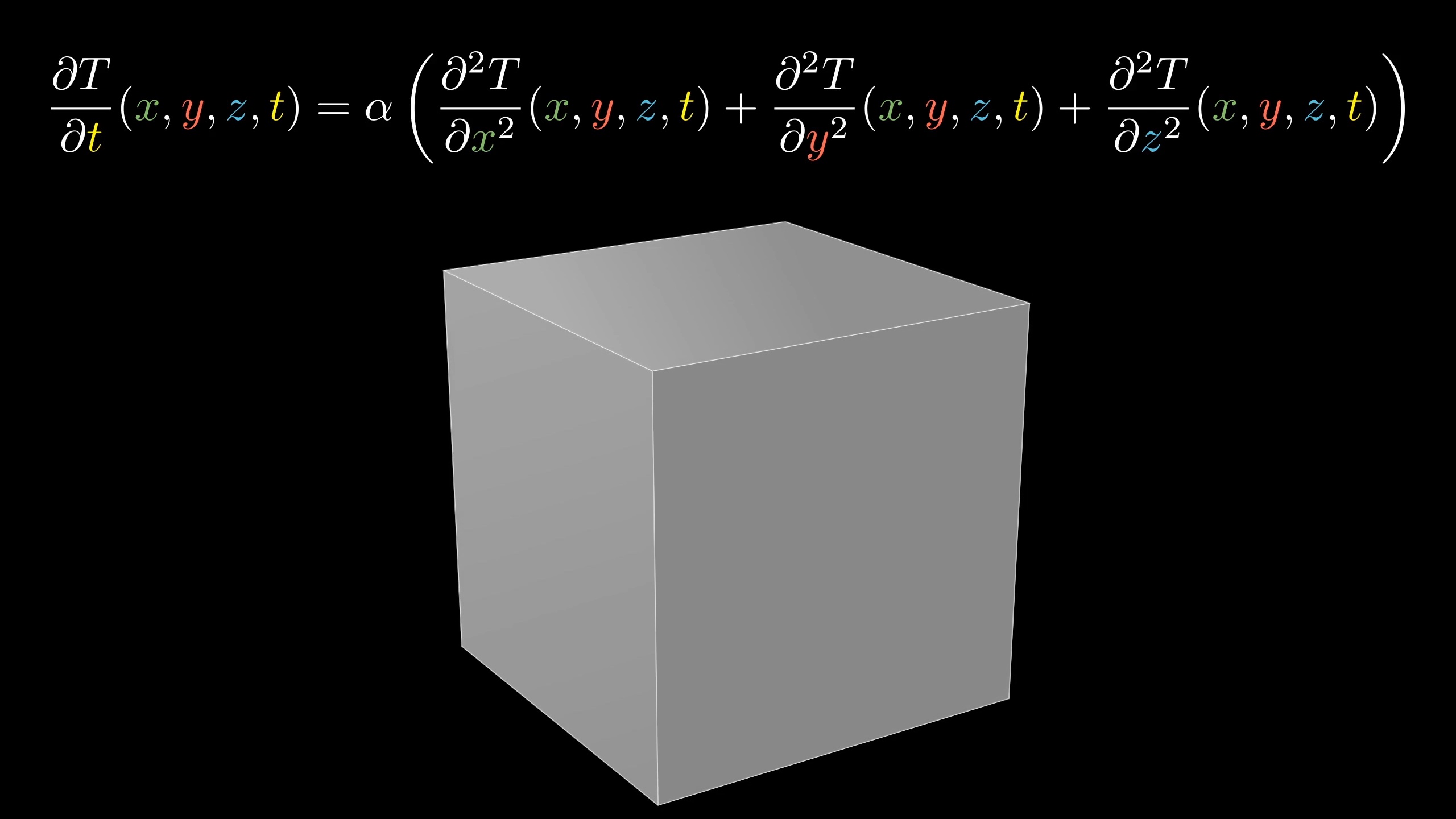
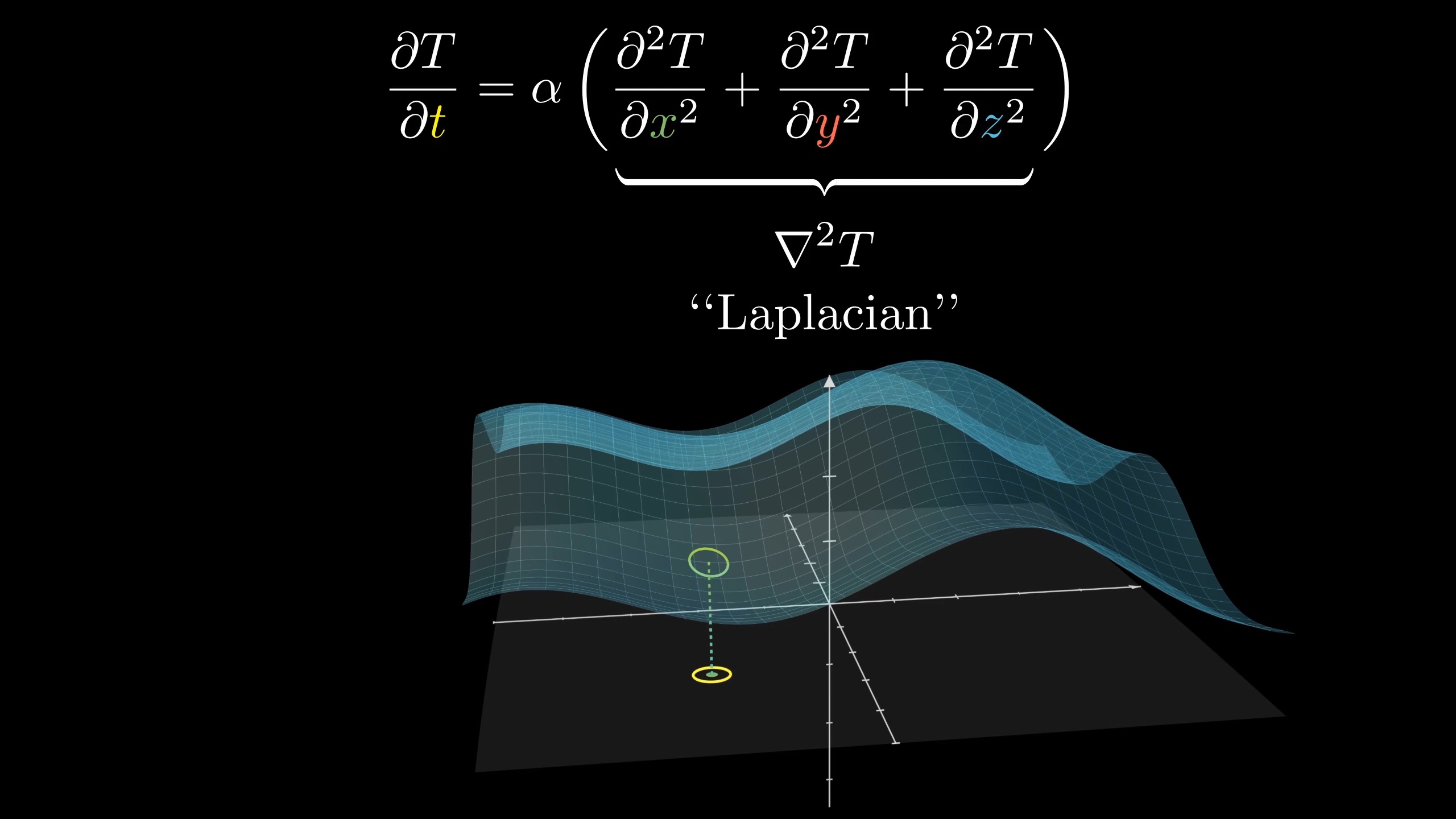
When your object is spread out in more than one dimension, like a plate, or a cube, the equation looks quite similar, but you include the second derivative with respect to the other spatial directions as well.

Adding all the second spatial second derivatives like this is a common enough operation that it has its own special name, the “Laplacian”, often written as an $\nabla^2 T$.

It’s essentially a multivariable version of the second derivative, and the intuition for this equation is no different from the 1d case: This Laplacian still can be thought of as measuring how different a point is from the average of its neighbors, but now these neighbors aren’t just to the left and right, they’re all around.

I did a couple of videos during my time at Khan Academy on this operator, if you want to check them out. For our purposes, let’s stay focused on one dimension.

Next lesson

If you feel like you understand all this, pat yourself on the back. Being able to read a PDE is no joke, and it’s a powerful addition to your vocabulary for describing the world around you. But after all this time spent interpreting the equations, I say it’s high time we start solving them, don’t you? And trust me, there are few pieces of math quite as satisfying as what poodle-haired Fourier developed to solve this problem. All this and more in the next chapter.